11.0 Overview
Vision is a process that feels relatively effortless to humans but that is very difficult for computers (Ballard et al, 1983).
This chapter explains the four areas of computer vision technology that have had the most impact on real-world applications. These are illustrated below:
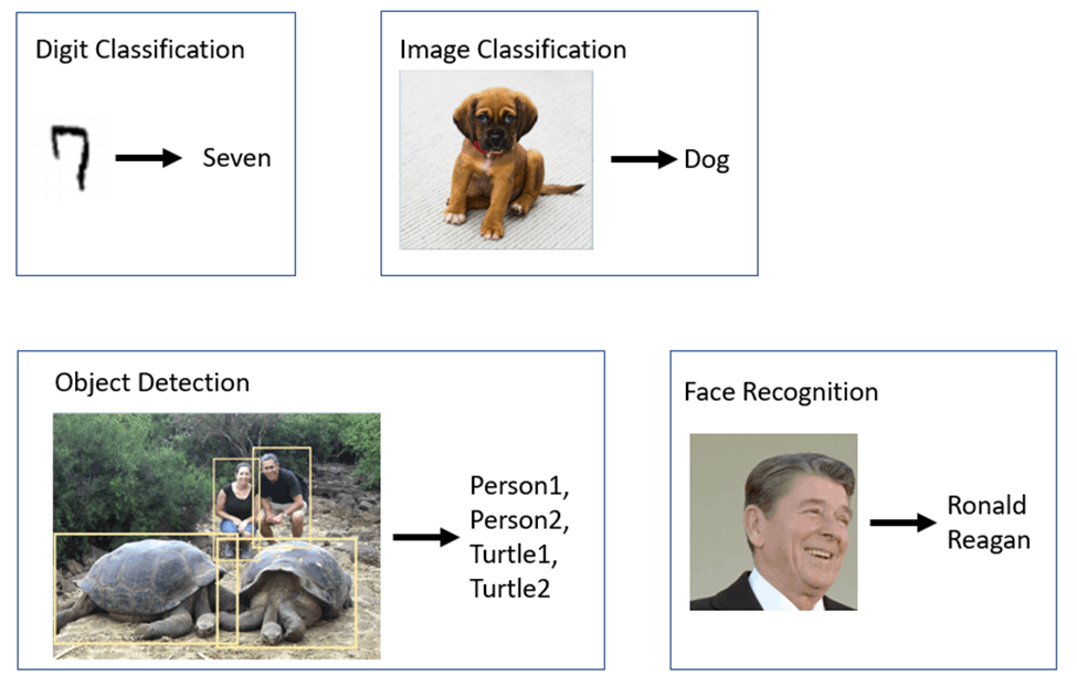
The four areas are:
Handwritten Digit Classification: Identifying digits such as handwritten zip codes.
Image Classification: Identifying the primary category (e.g. dog, flower, …) in an image even if the image contains multiple objects.
Object Detection: Localization and classification of multiple objects in an image.
Facial Recognition: Identifying the name of the person in an image.
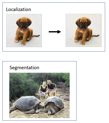
Note: Localization refers to identifying a bounding box for each object in the image as illustrated below:
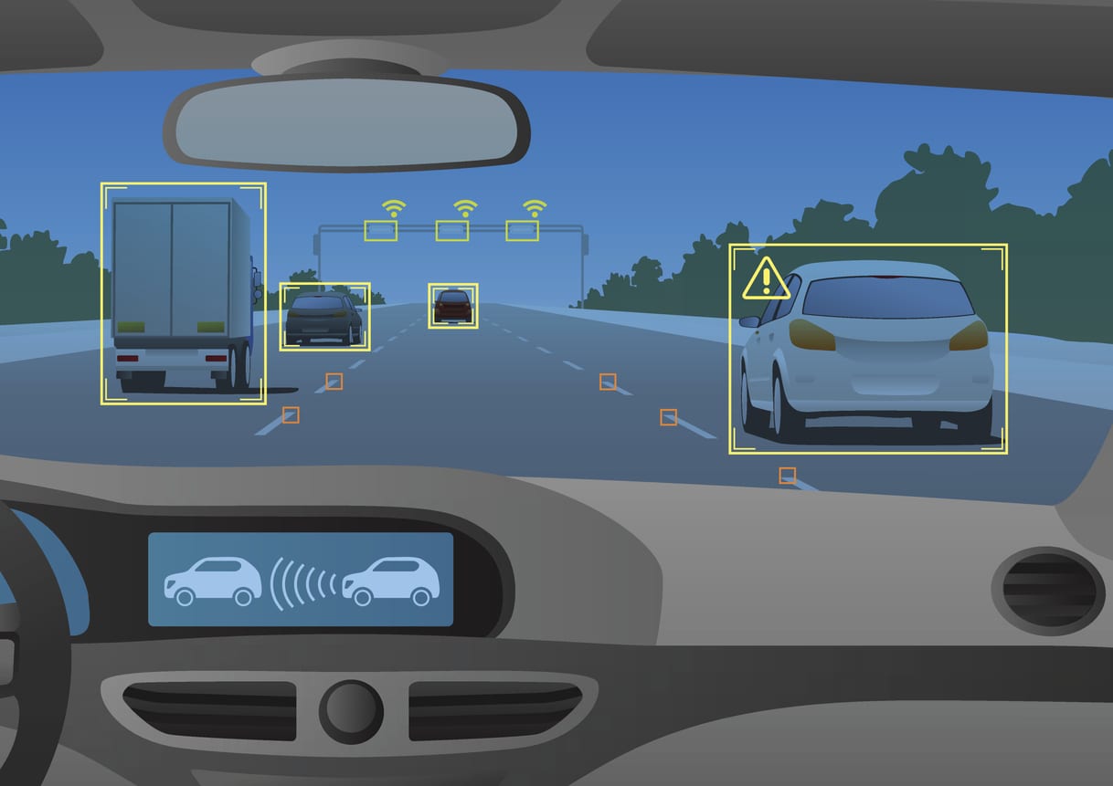
Applications of these computer vision technologies are numerous and include autonomous vehicles, traffic management, medical diagnosis, sports analysis, industrial automation, and security to name just a few. Computer vision researchers also work on building systems for many related tasks, most of which make use of methods similar to the ones discussed in this chapter.
Computer vision researchers also break these tasks down into smaller tasks such as image localization and image segmentation. These tasks are often studied separately with the idea that solutions can be used to improve performance on other vision tasks.
11.1 Handwritten digit classification
One of the early successful applications of computer vision technology was the recognition of handwritten numbers. Handwritten digit classification was a major priority of the US Postal Service for many years.
Yann LeCun and colleagues at Bell Labs in New Jersey studied this problem extensively in the 1990s. In 1990, they (LeCun et al, 1990) acquired a database of 9298 handwritten digits from the Buffalo, NY post office plus 3349 printed digits in a variety of fonts. They used a convolutional network (CNN) with 3 layers and a total of 4635 neurons and achieved an error rate of 3.4%.
In 1995, they (LeCun et al, 1995) created the MNIST database that has 60,000 training and 60,000 test images of 20×20 pixel handwritten digits. Their LeNet-5 CNN was a 7-layer network with 2 convolution layers. It achieved an error rate of 0.9%. In 1998, these computer vision researchers (LeCun et al, 1998) increased the size of the training set by adding automatically generated distorted versions of the digits. These distortions included transformations such as horizontal and vertical translation, scaling, squeezing, and shearing. The added training items reduced the test set error rate to 0.7%.
The MNIST database has been used in a great deal of research since then. In 2013, Wan et al (2013) lowered the error rate to 0.21%. The chapter on deep learning explained how a feedforward network could be used to recognize handwritten digits like those from MNIST and that chapter contains sample code for a CNN for recognizing handwritten digits.
Another heavily used digit database is the SHVN dataset that contains 600,000 images from house numbers in Google Street View images. It comes in two formats. One format is single digits – like MNIST – however, many images have some distractors. The other format is the original image with bounding boxes around each image so that boundary detection is easier.
11.2 Image classification
Perhaps the most widely studied computer vision subfield is image classification. The goal is to take an image and identify the category of the image (e.g. dog, flower, …). There are many applications of image classification technology from autonomous driving to generating audio captions of images for visually impaired users.
Neural networks are now the dominant technology for image classification. Prior to the advent of neural networks, image classification (and most other image processing tasks) used a pipeline approach that is described below.
11.2.1 Supervised learning using feature extraction methods
The first step in the typical pipeline is image preprocessing. Here, the image is cleaned up and transformed to the same size and shape as all the other images.
One of the earliest and best-known feature extraction technique is the Scale Invariant Feature Transform (SIFT) (Lowe, 1999). SIFT uses filters on images to extract a set of features that are invariant to image scaling, translation, rotation, reflection, and (to some degree) illumination.
Another heavily-used type of feature is Histogram Of Oriented Gradients (HOG)(Dalal and Triggs, 2005). HOG breaks an image into small regions known as cells and to create a histogram of gradient directions or edge orientations over the pixels of the cell. After some normalization, these histograms can serve as features that are input to a classifier (e.g. an SVM).
Other feature extraction methodologies include Speeded Up Robust Features (SURF) (Bay et al, 2006) and HAAR features (Viola and Jones, 2001).
There has been a significant amount of research effort put into enhancing the SIFT and HOG methodologies to develop better image feature detectors using techniques such as deformable part models (e.g. Felzenszwalb et al, 2010) and a high-level representation termed the Object Bank (Li et al, 2010).
Probably the most heavily-used technique for turning these features into inputs for machine learning algorithms is the bag of visual words (BOVW) developed independently by Sivic and Zisserman (2003) and Csurka et al (2004). The idea is to classify images similarly to the way text is classified using a bag of words as the input features. The words, in this case, are visual features identified by taking a low-level set of feature vectors (e.g. SIFT features) and clustering them to find the visual features. Then histograms showing the counts of these clustered features in each image are used as input to a classification algorithm such as an SVM or k-Nearest Neighbors.
Classifiers based on these types of features have been shown to be effective on datasets with large numbers of categories. For example, the WSABIE model (Weston et al, 2011) was able to process a dataset with 16,000 ImageNet categories. This is approaching human performance which is thought to be around 30,000 categories (Biederman, 1987). However, only 10% of the images were correctly labeled.
Weston et al also demonstrated the algorithm on web images with 109,000 categories but with much lower performance. Sánchez et al (2011) were able to improve the correctly labeled image percentage to 16.7% and Perronnin et al (2012) to 19.1%. Three issues should be noted for this type of classifier:
- As the number of categories in an image classification task increases, performance for most algorithms decreases (Deng et al, 2010). This is not surprising as one would expect performance to be higher when the categories are visually dissimilar and lower when the categories are visually similar. The more categories in a classification task, the higher the likelihood that there will be visually similar categories.
- The classifiers that perform best on smaller datasets might now perform best on larger ones. Deng et al (2010) showed that a linear SVM outperformed a k-Nearest Neighbor classifier for a dataset with a smaller number of categories but k-Nearest Neighbors outperforms on a large (10,000 category) dataset.
- The classifiers are learned specifically for a task. For example, Dalal and Triggs studied pedestrian detection (i.e. pedestrian vs no pedestrian classification). So, for this task, a set of labeled images with pedestrians and a set of images without pedestrians had to be collected. However, this classifier would not help with the detection of pedestrians in crosswalks vs. pedestrians on the sidewalk. This task would require a new set of images labeled with crosswalk vs. sidewalk.
11.2.2 Deep learning
The most widely used dataset for image classification research is ImageNet which was created by Princeton University researchers (Deng et al, 2009). ImageNet is a dataset of images organized according to their WordNet (Miller, 1995) hierarchy.
It has over 14 million images for over 21,000 of the WordNet synsets. There are an average of 650 images per synset. There are 27 high-level categories such as appliance, bird, and flower and each high-level category has numerous subcategories (e.g. the bird category has pigeons and other types of birds). Images can contain multiple objects. Each image contains an average of 1.5 objects.
The ImageNet Large Scale Visual Recognition Challenge (ILSVRC) is an annual image classification and segmentation competition started in 2010. The ILSVRC dataset is a subset of ImageNet that contains approximately 1000 images in each of 1000 categories. There are a total of 1.2 million training images, 50,000 validation images, and 150,000 test images.
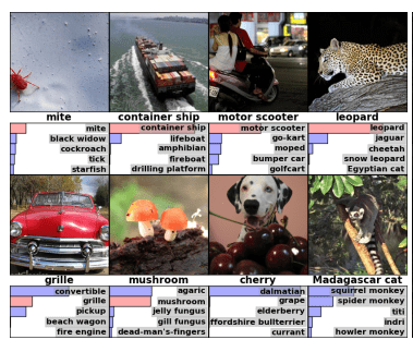
The primary measure used in the competition is the top-5 error rate which is the percentage of test images for which the correct label is not found in the top 5 predictions of the model. Top-5 means that the correct category was one of the system’s top five predictions of the category for each image as illustrated below.
Many university and commercial teams have participated over the years with 35 teams in the 2010 competition and 172 teams in the 2016 competition. Progress on the ILSVRC image classification task has been dramatic and is illustrated below:
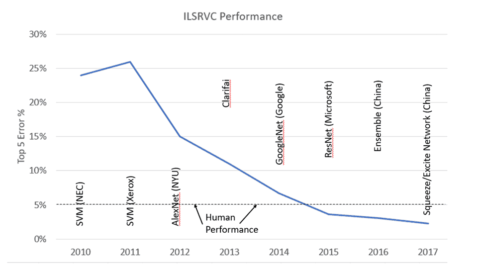
In the first two competitions, the two different winners used different types of feature extraction (e.g. SIFT) plus SVM classification to achieve a 28% top-5 error rate in 2010 and 26% in 2011. The error rate for the top prediction was 47% in 2010.
The 2012 competition woke up the world to the power of neural networks in general and CNNs in particular. AlexNet was created by a team of University of Toronto researchers (Krizhevsky et al, 2012). It won the 2012 challenge by achieving a 15% top-5 error rate. The next best system achieved only 26%! (It should be noted that the AlexNet top-1 error rate was still around 37%).
AlexNet had 5 convolutional layers, 60 million parameters, 650,000 neurons, and a 1000-neuron final layer that did the 1000 category classification. The Alexnet advances included efficient use of GPUs, use of the ReLU activation function, use of dropout layers to reduce overfitting, and use of techniques to add additional images to the training set by transforming existing images (e.g. rotating, translating, and zooming in/out). The AlexNet architecture builds on the LeNet-5 architecture discussed above and is a series of convolution layers followed by max pooling layers. At each step, the network is believed to learn higher and higher-level features. Subsequently, other research teams built CNNs with more layers as illustrated below:
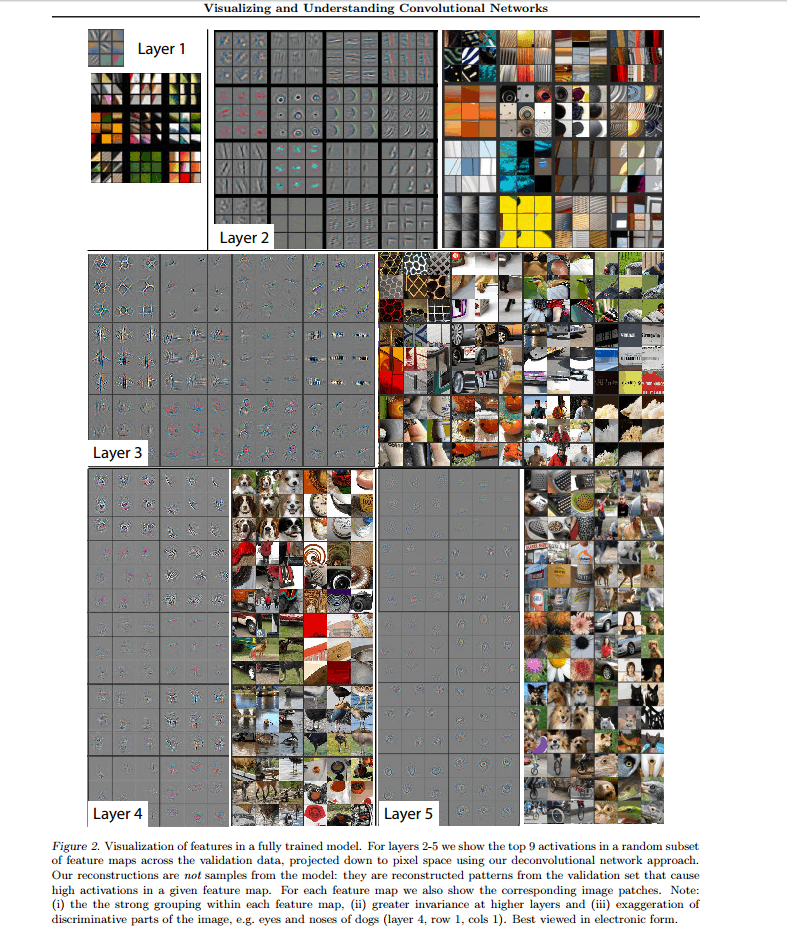
A New York University team (Zeiler and Fergus, 2014) developed a visualization technique termed a deconvolution network. The deconvolution network essentially turns the features in the hidden layers into pictures (pixels) and enables visualization of what is happening internally in the CNN layers.
By using this technique in the AlexNet architecture, the research team was able to fine-tune the architecture and produce a lower error rate. At the time, Matt Zeiler was an NYU Ph.D. student. When he finished his degree, he was reportedly offered millions of dollars by tech giants such as Google, Facebook, and Apple. Instead, he found a company, Clarifai, that is still independent and has raised about $100 million in capital as of Aug 2022.
The 2013 competition was won by a Clarifai entry with a top-5 error rate of 11%.
The 2014 competition saw several new architectures that are still used today. Two University of Oxford researchers (Simonyan and Zisserman, 2015) created the VGG16 model which had 16 convolutional layers and achieved a 7.3% top 5 error rate and is now widely used for image classification tasks.
The 2014 competition was won by a team of Google and academic researchers (Szegedy et al 2014b). Their GoogLeNet system (also known as Inception V1) achieved a top-5 error rate of 6.7%. The GoogLeNet architecture has 22 layers. Russakovsky et al (2015) looked at the top-5 performance of two expert human annotators. The better annotator achieved a top-5 error rate of 5.1% which was only slightly better than GoogLeNet.
A blog post by Andrei Karpathy (2014) analyzed the types of errors made by GoogLeNet vs. humans. GoogLeNet makes more mistakes with:
- Small and/or thin objects
- Objects in images enhanced with photographic filters
- Objects in abstract images such as paintings and sketches
- Extreme closeups
- Rotated objects
- Objects with identifying text
- Occluded objects
In contrast, people made more errors with:
- Fine-grained sub-categories such as identifying the type of dog
- Class unawareness. Human annotators weren’t always completely aware of all 200 classes.
- Insufficient training data. Human annotators saw only 13 examples of each class and sometimes this wasn’t enough information.
In 2015, Microsoft reported that its ResNet system achieved a 4.9% error rate (He et al, 2015a) using a very deep architecture with 152 layers. The authors pointed out that their system was the first to achieve human-level performance by comparing their result to Karpathy’s 5.1% estimate of human performance. It should be noted that the top-1 error rate of the ResNet system was still over 20%.
The 2015 ImageNet Challenge was won by a Microsoft entry (He et al, 2015b) that was an ensemble of ResNets that achieved a top-5 error rate of 3.57%. The top-1 error rate was still over 19%.
In 2016, a team from the Chinese Ministry of Public Security achieved a 3% top-5 error rate by using an ensemble of networks including Inception, ResNet, and Wide Residual Networks (Zagoruyko et al, 2017). That entry barely beat a Facebook team that achieved a 3.03% top-5 error rate.
The 2017 (and final) challenge was won by the “Squeeze-and-Excitation” network created by another group of Chinese researchers (Hu et al, 2018) with a top-5 error rate of 2.25%.
Many CNN were developed post-AlexNet through 2018. A group of researchers (Bianco et al, 2018) summarized the size and performance of many of those systems in the diagram below:
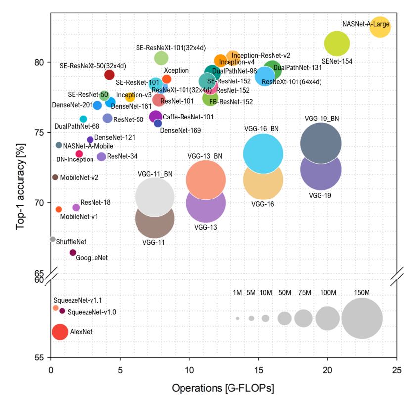
More recently, researchers have shown that transformer architectures for image classification can be as or more effective than CNNs. For example, Google researchers (Dosovitskiy et al, 2020; Zhang et al, 2021; Li et al, 2022) used a Vision Transformer instead of a CNN to successfully classify images. Even more impressive results were obtained with the Swin Transformer (Liu et al, 2021). Other Google researchers have been able to obtain good results with a plain of multi-level perceptron model (Tolstikhin et al, 2021). However, there is some evidence that the superiority of transformer models over CNN models is just do to better training methodology (Liu et al, 2022).
Vision transformers have also been used to convert 2D images to 3D scenes (Božic et al, 2021), to facilitate object detection in 3D point clouds (Wang et al, 2022), and to predict video frames (Gupta et al, 2022).
11.2.3 Self-supervised learning
One challenge with supervised learning is finding/creating sufficient labeled examples. Because images have to be labeled by hand, millions of labeled images are available but not billions.
Self-supervised learning, which doesn’t require labels, can also be used for images. Autoencoders and general adversarial networks use unsupervised learning techniques that take a sample image as input and reconstruct the image on output. Google DeepMind researchers (van den Oord, 2016a) developed the PixelRNN and PixelCNN models that generate images pixel by pixel.
Essentially, the value of each pixel in an image is a distribution based on the pixels that precede it in its row and on pixels in rows above it. By predicting the image pixel-by-pixel, the resulting generated images are sharp and coherent.
OpenAI researchers (M. Chen et al, 2020) showed that transformers using autoregressive modeling using learn strong image representations. They pretrained a GPT-2 model to predict pixels. When the pre-trained model was fine-tuned on ImageNet, the system achieved 99% accuracy in image classification which was comparable to system pre-trained with supervised learning.
In Chapter 4, there was a discussion of an unsupervised contrastive predictive coding system named SimCLR to pre-train a model and then achieved very good results on the ImageNet dataset by supervised fine-tuning on the pre-trained model with just 1% of the ImageNet training examples.
Another group of researchers (Fernando et al, 2017) presented the system with sequences of frames from a video. In each sequence, one frame was randomly inserted and therefore did not belong. In the example below, both sequences of frames show a boy jumping into a water hole. However, the first set of frames is in the correct order, the second set is in the wrong order.

The system was trained to identify the “odd-one-out” frame. The learned representation was then fine-tuned with training examples in which the label for each frame sequence was the name of the action portrayed in the frame sequence. The resulting model outperformed the previous state of the art by 12.7%.
Another SSL approach (Doersch et al, 2015) is to start with a database of images and broke up each image into 9 parts as illustrated below…
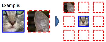
Each input was the middle part plus one of the other 8 parts and the model was trained to predict the location of the part (e.g. top-left, top-middle, …). By learning to do this, the model was able to learn enough about images to be able to classify all images of cats as a class of objects, all images of people as a class of objects, and the same for other object types.
Companies such as Google (Waymo) and Tesla use cameras and other sensors in cars to correlate user driving actions to sensor input. The AI systems learn to produce the actions of the drivers given the sensor input. The driver actions are in effect the labels for the data for further information on autonomous vehicles. For more information on this topic, see the chapter on autonomous vehicles in my book or see this blog post.
A group of DeepMind researchers (Grill et al, 2020) created yet another SSL approach they named Bootstrap Your Own Latent (BYOL). BYOL uses two networks, an online network and a target network. The online network predicts the target network representation of an augmented image under a different augmented view of the same image. Then it updates the target network with a slow-moving average of the parameters of the online network. A linear classifier trained on the frozen BYOL representation yielded a 79.6% top-1 accuracy on ImageNet.
Barlow Twins (Zbontar et al, 2021) is another SSL dual-network approach.
Contrastive methods such as the one used to train SimCLR are computationally expensive because they require large numbers of pairwise feature comparisons. Facebook researchers (Caron et al, 2021) developed SwAV which avoids the pairwise comparisons by using a cluster technique by ensuring that different views of the same image get assigned to the same cluster.
Most SSL research has centered around the ImageNet dataset. To determine if these SSL techniques work more generally, Facebook researchers (Goyal et al, 2021) pre-trained a model on billions of random internet images. Their model, SEER, used SwAV to pre-train a model. Then, when the model was fine-tuned on ImageNet, it achieved a top-1 ImageNet accuracy of 84.2%. With fine-tuning on only 10% of ImageNet, they achieved 77.9% accuracy.
Visla and Hugging Face both offer open source libraries for image training via SSL.
11.2.4 Semi-supervised learning
Researchers have had some success with semi-supervised image classification approaches that reduce the need for massive labeled datasets. OpenAI researchers (Salimans et al, 2016) trained a Generative Adversarial Network to generate images from the same distribution as a training set of images and additionally trained the Discriminator to output an image label.
The new images with the labels were then added to the training set. The result was good performance on several different datasets (including ImageNet) with a small set of manually labeled examples. Facebook researchers took a different approach. The first step was to train a model on a limited amount of labeled data. The training examples were then ranked for each concept class and the top-scoring examples selected for each class. Then the top examples were used to train a new model and this new model was fine-tuned on all the existing training data. The resulting model outperformed a model trained solely on the labeled data.
Noisy student training (aka self-training) was used by researchers (Xie et al, 2020) to achieve a state-of-the-art top-1 accuracy of 88.4% on ImageNet. They started with a network that was trained on ImageNet. Then, they used that network to predict labels for 300 million unlabeled images. They selected the predicted labels that had a medium-to-high confidence rating. They then used that model as a teacher model to train a student model. Noise was created in the student model using three technique: First, they randomly removed layers using a technique known as stochastic depth (Huang et al, 2016). Second, they randomly removed nodes using a technique known as dropout (Srivastava et al, 2014). Third, they used random augmentations of the images using a technique named RandAugment (Cubuk et al, 2019).
11.2.5 Weakly supervised learning
Facebook researchers (Mahajian et al, 2018) collected billions of images from Instagram labeled with hashtags. They matched 1500 of the hashtags with ImageNet categories and trained a CNN-based classifier to classify images into their hashtag categories and achieved an ILSVRC state of the art top-5 error rate of 2.4% and a top-1 error rate of 14.6%.
Facebook researchers also developed a classification algorithm that combined semi-supervised and weakly-supervised learning and worked better than either.
11.3 Object detection
Object detection is similar to, but more difficult than, image classification. In image classification, the goal is to identify the category of the primary object in the image. In image classification datasets, most images have only a single prominent object. In contrast, the object detection task is to find all the objects in an image and classify them.
Like image classification, earlier object detection architectures typically involved feature extraction plus training on those features to build a model. More recently, all-in-one deep learning architectures do both at the same time.
11.3.1 Datasets
The ImageNet dataset images on average contain one and a half objects (some contain just one object, some two, some three, and so on).
The PASCAL Visual Object Classes (VOC) dataset (Everingham et al, 2009) was created prior to ImageNet, served as the basis for an annual challenge from 2005 through 2012, and is still commonly used as a benchmark for object detection research. It initially had just 4 classes. The VOC 2012 benchmark has 20 classes, 11,500 images, and 27,500 detection objects (of which 6,900 have bounding boxes).
The ImageNet competition also included an object detection challenge from 2013 through 2017 that was harder than the VOC object detection task because the ILSVRC dataset has many more categories. The ILSVRC 2013 dataset has 345,000 objects in 395,000 images in 200 categories. It was expanded to include more objects and images in 2014.
The Caltech Pedestrian Dataset (Dollár et al, 2012) that includes 350,000 pedestrian bounding boxes labeled in 250,000 frames.
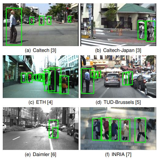
11.3.2 Supervised learning approaches
Supervised learning approaches to object detection use one of two methodologies. In two-stage methodologies, the first stage identifies the bounding boxes and the second stage classifies the images inside the bounding boxes. In one-stage methodologies, both are done at the same type which results in faster production use.
An example of a two-stage method is the R-CNN architecture (Girshick et al, 2014; Girshick, 2015; Ren et al, 2016) which does the following:
- Identify the bounding boxes (termed “regions”) for each object. They used a technique known as selective search (Uijlings et al, 2013) produced around a relatively small number (e.g. 2000) hypothetical regions for each image. The selective search technique works better than earlier methods that used an exhaustive search of each image. It identifies small candidate regions using color and contour similarity metrics and merges them hierarchically into larger and larger candidate regions.
- Use a pre-trained image classifier to extract a fixed-length feature vector for the pixels in each region.
- Use these features as inputs to an SVM classifier for each category.
They termed this method R-CNN for “regions with convolutional neural network features”. This method achieved an mAP of 54% on the VOC 2010 dataset compared to a previous best of 33% using HOG features in a deformable part model.
YOLO (Redmon et al, 2016; Redmon and Farhadi, 2017; Redmon and Farhadi, 2018; Bochkovskiy et al, 2020), which stands for You Only Look Once, is a single-stage method that uses a single CNN to simultaneously identify multiple bounding boxes and classify the images in those bounding boxes. It does this by learning the pixel-by-pixel probabilities of each bounding box and image class.
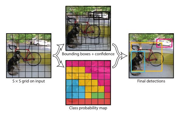
As illustrated above, YOLO works by first imposing a grid on an image. Each grid cell is responsible for learning both the probability that it is inside a bounding box and the probably of the image category within the bounding box.
Historically, CNNs have been the dominant architecture for object detection. More recently, transformers such as the Swin Transformer (Liu et al, 2021) have shown the ability to outperform CNNs.
11.3.3 Unsupervised object detection
Researchers have found several unsupervised methods of reducing the reliance on labeled images for computer vision tasks such as object detection and image classification.
One interesting approach was devised by two Carnegie Mellon researchers (Wang and Gupta, 2015). They started with 100,000 videos pulled from the web. Their idea was that a patch (a square subset of an image) from one frame of a video is likely to hold the same object or object part in the next frame of the video.
They used a CNN to learn an image similarity model in which the similarity of the patches in two sequential frames is greater than the similarity of patches in two random frames. The final CNN layer is a set of weights that serve as the features of the image.
They then used the final layer weights to create clusters of training images using a nearest neighbor algorithm. Each cluster is an object. The learned model can then serve as an image classifier. The classifier takes a test image as input, is run through the network, and is classified according to its nearest neighbor. So, they effectively built an object detection algorithm with no supervision. Their systems performed almost as well as a baseline supervised learning system.
1
1.3.4 Compositional object detection
Image classification is often viewed as a machine learning problem in which the objective is to find patterns in a set of input examples that can correctly distinguish amongst a finite set of categories.
One problem with this approach, as discussed above, is that adding categories requires many new examples and re-training. In contrast, people can learn to classify new categories with one or relatively few examples.
A second problem with this approach is that the extension to object detection and scene analysis in which there are multiple objects in a scene then relies on a separate algorithm that finds bounding boxes around the individual objects.
A compositional approach to object detection in scenes is to view each category as composed of parts. For example, a dog has a head, a tail, and four legs. The parts have sub-parts. A head has eyes, ears, a nose, and a mouth. A dog can be distinguished from a horse or a cat by the relative sizes of the parts, the spatial arrangement of the parts, and specific characteristics of the parts. A horse’s head has a different shape and arrangement of eyes, ears, nose, and mouth than does a dog’s or a cat’s head.
The idea of a compositional representation of objects in humans has a long history (e.g. Biederman, 1987). The idea was illustrated by a 2006 Brown University study (Jin and Geman, 2006). These researchers built a system for reading Massachusetts license plates with 98% accuracy. At the lowest level, the system detected predefined parts of characters and parts of plate sides. At the next higher level up, probabilistic functions were created that mapped the probabilities of each character and plate side to the predefined parts. Then these higher-level features were used to create even higher-level features until, at the highest level, license plates were identified. In this system, the probabilistic maps from lower to higher levels were hand-crafted; however, as the authors noted, they could have been learned.
Historically, even compositional object detection systems have been task-specific, and learning new categories requires many additional examples and re-training. Fidler et al (2008) suggested that one path toward more general object detection is to have object categories that decompose into part hierarchies that have common elements at their leaf levels. Then, to recognize a new category, one would only need to learn how the leaf-level parts can be combined to compose examples of the category.
UCLA researchers (Kokkinos and Yuille, 2011) proposed that the leaf levels are tokens that are a set of straight edge and ridge segments. Tokens combine to form contours that combine to form parts that combine to form objects. Each object can then be defined by a grammar. Object detection is a process of composing lower-level features into higher-level features.
They showed that this methodology can handle deformed, occluded, and poor resolution images by achieving state of the art results on the UIUC car dataset which is a dataset of cars with very poor resolution and the ETHZ shape dataset which has deformed and occluded shapes.
Lake et al (2015) decomposed handwritten symbols into a set of strokes. By recognizing symbols based on strokes, their system was able to demonstrate the learning of new symbols with just a few examples.
A group of Vicarious AI researchers (Stone et al, 2017) looked at compositionality at the object level. They argue that for a CNN to provide a generic object detection capability, the activations of an object should be able to be transferred to a different object detection domain. For example, if one trains a CNN to recognize an airplane in a scene, the activations in the network that correspond to the learned features of the airplane should be the same whether the airplane is occluded or not in the scene.
Using a visualization technique, they were able to show that this is not the case for standard CNNs. Instead, the activations included elements of the occluding objects.
They used a set of CNNs with shared weights. One CNN was fed the original images with multiple objects. There was an additional CNN for each image category. The images fed into these additional CNNs were images with the other objects masked. They used an objective function that both minimizes overall classification loss and additionally penalizes the CNN if the activations of occluded and non-occluded objects are different. They showed that this architecture produces better results than just a single standard CNN.
11.4 Facial recognition
Facial recognition is a computer vision subdiscipline that has a great deal in common with image classification but it has a set of unique challenges. For example, below are four different images of former US President Ronald Reagan:
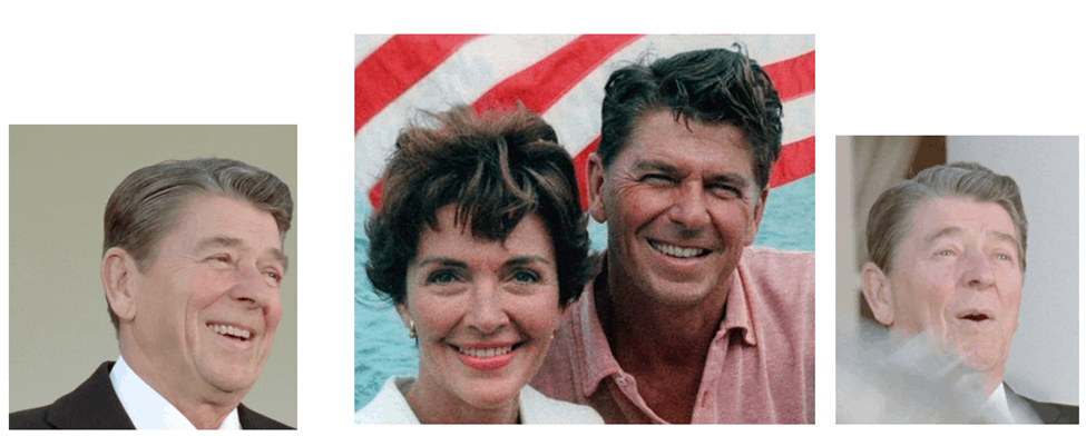
These three different images of the same person shows some of the challenges specific to facial recognition. Images of the same person can vary in pose (i.e. the 3D rotation of the face), lighting conditions, facial expressions, occlusions (the image on the right has a turkey wing partially obstructing the face), ages (Reagan is pictured as both a younger and older man), resolution, scale, and make-up. Other examples are disguise, orientation, and the presence of glasses, hats, and jewelry.
Additionally, many images (e.g. the middle image above) have multiple faces and/or other objects. Before facial recognition can be applied to these images, the bounding box must first be identified using Face Detection technology.
Face Detection is a special case of object detection discussed earlier in this chapter. Face Detection is a fairly mature technology at least for frontal images. The technology (Viola and Jones, 2001; Osadchy et al, 2007) is the basis for the autofocus feature in point-and-shoot cameras and smartphones.
Facial recognition systems typically operate in one of two modes: identification or verification. In an image identification system, there is a database of labeled images and the task is to determine if an input image is one of the images in the database. This is critical in applications like surveillance where one might want to determine if an input image matches an image in a terrorist database or an image in a mug book.
In contrast, image verification is about determining if two images are of the same person. Applications of image verification include unlocking a smartphone using one’s face, passport control, and verifying identity for access control purposes. Photo apps like the ones offered by Google, Apple, and Facebook use image verification to group photos of the same person.
The development of facial recognition technology has paralleled that of image classification. Prior to the use of deep learning in image classification, most facial recognition systems used a two-stage process (e.g. Chen et al, 2013):
- Derive a set of features (e.g. SIFT and HOG features) from the images that are invariant to pose, lighting, expression, and other intra-person variations.
- Apply a classification algorithm such as an SVM or linear discriminant analysis to distinguish the pictures of one person from another person.
In 2014, inspired by the success of AlexNet for image classification, Facebook researchers (Taigman et al, 2014) trained a CNN-based system named DeepFace on four million images of four thousand people and accuracy on a benchmark dataset named Labeled Faces in the Wild (G. Huang et al, 2007) to 97.35% which reduced the error rate by 27%.
Google followed shortly thereafter by training its FaceNet system on 200 million images of 3 million people and improved accuracy to 99.67% (Schroff et al, 2015). The CNN algorithms operate without pre-defined features and appear to do a better job of learning a set of features that represent faces in a form that is invariant to pose, illumination, and other sources of intra-person variation.
There are many commercial and open source face detection and recognition tools on the market such as Amazon’s Rekognition, Google’s Vision AI, and Microsoft Computer Vision product offerings.
11.5 What is being learned by computer vision systems?
A network that can be trained to classify images and exhibits relatively little increase in error from training to test can be said to have learned to classify the images.
But what has been learned? Has the network gained a deep human-like understanding of the different categories?
It is generally thought that the initial layers of CNNs for image processing tasks learn low-level features such as edges, lines, and curves. It turns out that most image processing tasks produce very similar initial layers. A group of vision researchers (Yosinski et al, 2014) noted:
“Modern deep neural networks exhibit a curious phenomenon: when trained on images, they all tend to learn first-layer features that resemble either Gabor filters or color blobs. The appearance of these filters is so common that obtaining anything else on a natural image dataset causes suspicion of poorly chosen hyperparameters or a software bug.”
These researchers also noted that as one progresses through the layers, the features tend to be more specific to the task.
When these early layers are extracted from a trained network and used to initialize a network for a different vision task, performance on the new vision task is increased, learning time decreased, and not as many training examples are required.
The question remains, however, whether these systems are learning the concepts underlying the image categories or whether they are just learning statistical regularities that are useful in classification.
A group of Google, NYU, and University of Montreal researcher (Szegedy et al, 2014a) set out to study this question. They trained a neural network on an image classification dataset. Performance on the test data showed strong generalization (i.e. very little increase in test error over training error). Then they created a set of adversarial test images with perturbations that were not visible to the human eye and didn’t affect the ability of humans to correctly classify the images. The idea was that, if the network really had a deep understanding of the image categories, the perturbations would not affect the ability to classify the images anymore than they affected the ability of humans to classify the images. However, they found that the network was far worse at classifying these adversarial examples.
Some other examples of adversarial attacks on computer vision systems:
- Adding random noise to images can cause them to be misclassified (Goodfellow et al, 2015).
- Placing post-it-like stickers on images of stop signs cause deep learning systems to lose the ability to classify the stop sign, i.e., to not “see” the stop sign. Yet, people have no trouble recognizing the perturbed image as a stop sign with a sticker on it (Eykholt et al, 2018).
- Just by modifying just a single pixel in an image, it is possible to alter an object recognition system’s category choice. In one instance, by changing a single pixel on a picture of a deer, the object recognition system was fooled into identifying the image as a car (Su et al, 2019).
- It is possible to make people invisible to person detection systems (i.e., systems that classify an image as a person but that do not identify the person). One group of researchers started with a full-length photo of a person, an image the system easily identified. Then, in another photo, the person held a colorful patch that just covered their waist but did not come near their face, and the system could no longer identify the person (Thys et al, 2019). A group of Russian researchers developed a card that they placed on a person’s hat that caused a facial recognition system to fail to identify the person wearing the hat. The card didn’t confuse people. University of Chicago researchers have developed a system named Fawkes that can inoculate images of oneself against facial recognition systems (Shan et al, 2020).
- Researchers have also figured out how to fool deep learning systems into recognizing objects such as cheetahs and peacocks in images with high confidence when there is no object whatsoever in the image(Nguyen et al, 2015).
So what is actually being learned? Two University of Montreal researchers (Jo and Bengio, 2017) created by a mathematical transformation that altered the surface statistical regularities of the images but that left them entirely classifiable by humans. They found that adversarial test images created in this fashion increased test error by 28%. They concluded that image classification networks do not learn high-level abstract categories. Instead, they learn surface statistical regularities. In the image below, adding a guitar causes the AI system to misclassify the monkey as human:
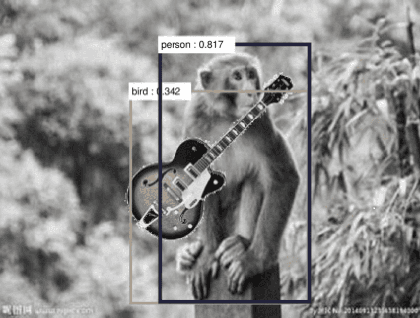
Another group of researchers (J. Wang et al, 2017) created adversarial test images by superimposing unlikely content. For example, they superimposed a guitar on a picture of a monkey. Humans have no problem recognizing this as a picture of a monkey with a guitar even though they’ve probably never seen an image of a monkey holding a guitar. However, neural networks classify it as a person not a monkey because all the training images they saw with guitars were labeled as people.
They take this as evidence that people have no problem decomposing the image into subparts but that networks don’t decompose and instead just learn the statistical regularities.
For a review of adversarial attack methods, see this article.
© aiperspectives.com, 2020. Unauthorized use and/or duplication of this material without express and written permission from this site’s owner is strictly prohibited. Excerpts and links may be used, provided that full and clear credit is given with appropriate and specific direction to the original content.