3.0 Overview

This chapter explains neural networks in general with a focus on the class of neural networks known as deep learning systems.

3.1 Why do we need deep learning neural networks?

Supervised Learning algorithms can be thought of as algorithms that learn a function relating the input variables to the output variables. Many supervised learning algorithms work well when the relationship is linear and some work well for minor deviations from linearity. However, when the underlying function is non-linear (and/or discontinuous) or there are large numbers (e.g. millions) of input variables, a neural network is often required.

3.2 Examples of deep learning networks

In this section, we’ll look at two examples of neural networks, one for the housing dataset discussed in the previous chapter, and one for recognizing handwritten digits.

3.2.1 Example: Deep learning network for the housing dataset

Let’s suppose we’re trying to predict housing values using the dataset described in Section 2.0. In that section, we discussed how we could use linear regression for this application. We could also use a neural network.  A simple neural network for this problem is illustrated below:

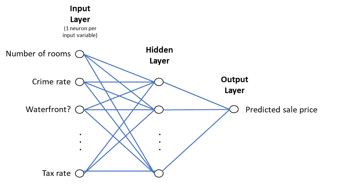
The input layer has one neuron for each input variable. You can think of neurons as variables, like the ones described above for the temperature and housing functions.

Neural networks also have weights that are like the weights for the temperature and housing functions. There is one weight for each connection between two neurons. In neural networks, the weights represent the strength of the connection between two neurons.

The output layer in the figure above has just one neuron that will contain the predicted sale price.

Each input neuron is connected to each neuron in the hidden layer. We use the term “hidden” layer because only the input layer and output layer values are derived directly from the training dataset. The term “hidden” is an unfortunate choice of terminology as it connotes something “secretive” or “unknowable.”

Each connection between neurons has a weight that starts off as a random number. To get the value of a neuron in the first hidden layer, one adds the values of all the connections to that neuron. The value of an individual connection is the weight of the connection times the value of the input neuron.

The connection weights are numbers just like the weight (with the value of 1.8) used in the Fahrenheit function above. The neurons play the same role as the input variable in the Fahrenheit function (i.e. the Celsius variable); however, neurons are more complex than a single variable as will be explained below.

If there is a second hidden layer, to get the values of the neurons in the second hidden layer, here again one adds the values of all connections to that neuron. This time, the value of an individual connection is the weight of the connection times the value of the first layer neuron to which it is connected. This process continues forward through all the layers of the network.

This type of network is known as a feedforward network. Here is the code in Keras for that network:

This code was written to predict the Kings Country housing values from the previous section. However, the same code could be used for a large number of supervised learning regression problems.

You’ll notice that there are no references to the housing data. The code snippet above just defines and executes the network model.

A complete program typically also contains preprocessing code to acquire the data and put it in the format required by the model (i.e. in the input_train and output_train matrices in the example above).

Keras offers two APIs. This example uses the Sequential model API which is the simpler of the two APIs and can only accommodate a linear stack of layers. The Functional API in Keras can be used to build most neural network models that you will find in the academic and commercial literature.

In the example above, the hidden layer and the output layer are each specified in a call to the .add method. A dense layer is a fully-connected layer (i.e. one in which each neuron is connected to all the neurons in the preceding layer and all the neurons in the following layer (except of course for the output layer where there is no following layer).

The first variable in the dense layer specifies the number of neurons. The first hidden layer (there is only one in the example above) must specify the number of input variables (or neurons) in the input_dim variable.

The .compile statement above specifies the cost function and the optimization method (see below) to use and creates the underlying parallelization code that makes use of multiple cores, CPUs, and GPUs.

The .fit statement is where the learning happens. The number of epochs specifies how many passes should be made over the entire training set and the batch_size specifies how many training items should be processed at a time (more on batch sizes below).

The processing of each batch is known as an iteration. If the batch size is the entire training set, then an iteration will be the same as an epoch.

Note on terminology: The term “iteration” has a specific meaning when applied to neural networks (i.e. the processing of the observations in a batch). The term “iteration” also has a more generic connotation when applied to algorithms in general (neural networks are a type of algorithm). In the general algorithmic sense, “iteration” means re-running a computation repetitively as a means of getting closer and closer to the desired result. You will see the term “iteration” used below in both the context of neural networks and in the context of other algorithms. The .predict statement takes as input the test input data and predicts the outputs (e.g. for the housing data it predicts the housing prices for the test data).

3.2.2 Handwritten digit classification

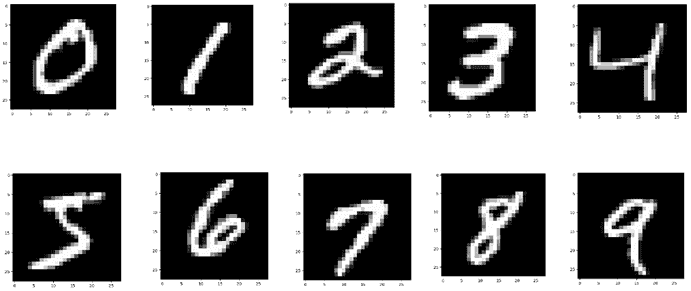
Now, let’s look at another example. Suppose we want to build a system that can recognize handwritten numbers like the ones below:

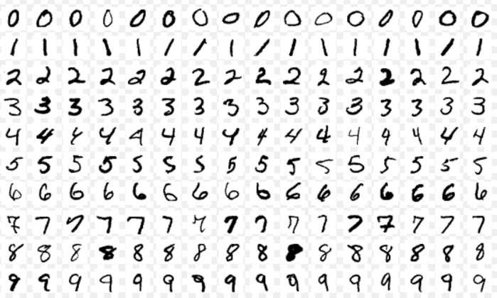
Source:  Josef Teppan licensed under CC BY-SA 4.0

These are images from an extensive database published by the National Institute of Science and Technology (NIST) in 1995 to support the development of handwriting recognition technology. Each image is 28 x 28 pixels. Pixels, short for picture elements, are the little dots that make up digital picture images.

For our training dataset, each training image will be a row. There will be one column for each of the 28 x 28 = 784 pixels plus a column for the output number. A neural network for this problem is depicted below:

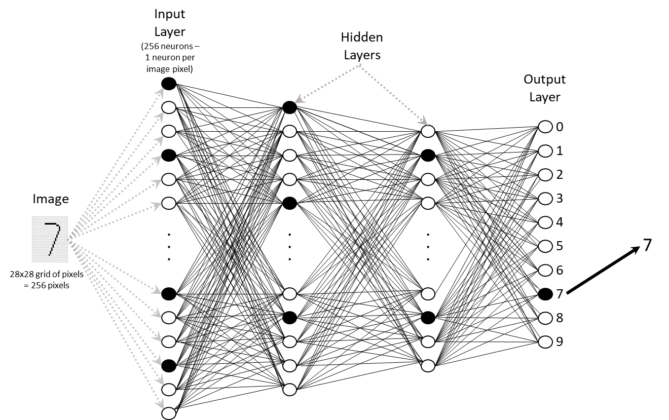
The network illustrated above has an input layer that has one neuron for each of the 784 pixels in the image of the handwritten number. Each of the 784 input layer neurons will have a value of one if it is black in the image and 0 otherwise.

The output layer has ten neurons, one for each possible output value (0-9). In the middle, there are two hidden layers.

We can write a function for this network (and for every neural network) that operates the same way as the function we discussed for computing Fahrenheit temperatures from Celsius temperatures. The difference is in the number of variables and weights in the function. Recall that the function for computing Fahrenheit temperatures is Fahrenheit = 1.8 x Celsius + 32.  There are two variables (the Fahrenheit value and the Celsius value) and one weight (1.8).

In contrast, functions that represent the computation in a neural network can have millions and even billions of variables and weights. Google’s T5 network had eleven billion parameters (weights). The job of a neural network algorithm is to learn the parameter values that best predict the output variable.

3.2.3 Why deep learning is revolutionary

As mentioned above, deep learning can succeed in computing very complex functions that generalize from the training dataset to the real world.  As a result, deep learning has a profound impact on our daily lives.  Deep learning networks recognize faces in our smartphone pictures, translate languages, and may soon drive our cars. Why do they work so well? 

AI pioneers Geoffrey Hinton and Yann Lecun (2021) argue that the primary reason is the growing computational capabilities that enable networks with many layers.  Research has shown that deep networks (i.e. those with many layers) outperform shallow network (i.e. those with fewer networks) even when the networks have the same number of parameters (Bengio, 2007). 

Hinton and LeCun believe that deep networks enable compositionality.  Specifically, features that are learning one layer are combined to create higher-level features in each next layer. They argue further that the human visual cortex displays a similar type of compositionality (Van Essen and Maunsell, 1983).

3.3 Computing the optimal weights

Recall that the Celsius to Fahrenheit function is Celsius = w1 * Fahrenheit + w2.  There is one weight, w1, and one parameter, w2, in this function. We know the optimal value of the weight is 1.8 and the optimal value for the parameter is 32. However, we’re going to again suppose we don’t know the optimal values and, instead of computing the values with a linear regression algorithm as we did in the supervised learning chapter, we’ll learn the correct values with an iterative algorithm, i.e. one that continually tries new values for the weight and parameter until it finds the optimal values.

3.3.1 Computing the function without a deep learning network

One way to iterate would be to write a computer program to try all values of w2 ranging from 1 to 100. Then for each value of w2, try values of w1 ranging from 0 to 1 in increments of .0001. As we try different values, we will keep track of the most effective values.

Let’s assume there are 100 rows of Celsius and Fahrenheit values in our training dataset. We will evaluate each choice of w1 and w2 by subtracting the correct Celsius value from the value generated by the function for each of these 100 examples.

The cost function will sum the absolute values of the these deviations for each of the examples in the dataset. After all the values for a and b have been tried, we will keep the values that produced the smallest error as defined by the cost function. This is a lot of calculations but modern computers can do this quickly. By doing so, we will get the correct answer of Fahrenheit = 1.8*Celsius + 32.

We didn’t need to use this brute force algorithm. A closed-form algorithm such as least squares would have worked fine. However, as the number of dimensions grows and/or the nonlinearity increases, the chances of finding a closed-form solution decrease. However, all data can be fit with a computational solution.

The most common computational optimization method used for neural networks is gradient descent.

3.3.2 Gradient descent

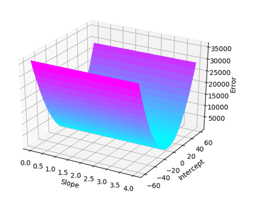
This section explains how to calculate the Fahrenheit function weights. Again, the goal is to find values of a and b that maximize the correctness of the formula Y = a*x + b.  The figure below shows a plot of the actual vs. predicted deviations (i.e. the Error) versus the slope and intercept for a wide range of slope and intercept values:

The goal is to find the lowest spot on this surface because that is where the error function has its lowest value.

Gradient descent is almost universally used to find the minimum on 2-dimensional surfaces like this one as well as on surfaces with many more dimensions.  The process of gradient descent will be described at a high level here skipping the math. A good source for the details on the math of gradient descent is this Coursera course.

Intuitively, if you look at the figure above and imagine the plotted values forming a terrain of sorts and image a ball rolling down the terrain. Gravity would cause the ball to stop at the lowest point in the terrain. Gradient descent is an iterative technique that works a lot like a ball rolling down the terrain.

It is an iterative technique in that you figure out which way is down, move a little in that direction and see if you’ve reduced the value of the cost function. When the value stops getting smaller, you have found the values that minimize the loss and that therefore offer the best predictive value for new data inputs.

Below is an example of using gradient descent for our Celsius to Fahrenheit example. Gradient descent will be used to determine that the best slope is 1.8 and the best intercept is 32.

The way gradient descent works for this example is to find the partial derivative of the cost function with respect to the slope variable and then again with respect to the intercept variable. A positive derivative value means that the error rate is increasing as the input variable (Celsius) increases. A negative value means its decreasing. The derivative tells us which way to move along the variable’s dimension in order to decrease the cost function.

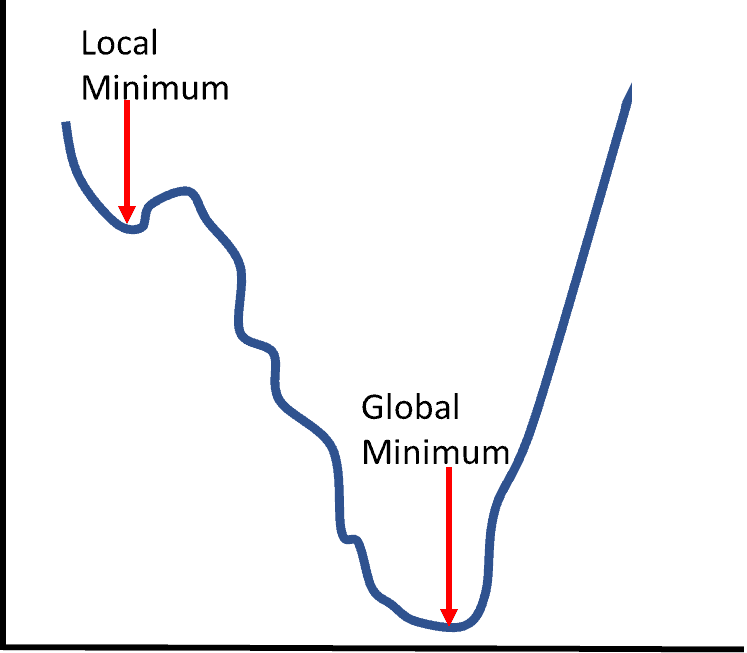
This technique works every time and computes quickly as long as the cost function produces a function that is convex (i.e. one in which a ball rolling downhill will always find the minimum as its resting point). In contrast, if the surface is non-convex, local minima can be a problem.

For example, if the surface is like the one in the figure above, a ball rolling downhill might get stuck in a local minimum rather than finding the global minimum.

As discussed below, there are a number of steps you can take to reduce the chances of this occurring. Interestingly enough, it turns out that getting stuck in a local minimum isn’t usually a disaster. It turns out that the majority of surfaces have multiple local minima that produce nearly the same values of the cost function as the global minimum.  Here is the sample code for this computation:

While gradient descent is by far the most common optimization methods, there are other interesting methods.

3.3.3 Initial weights

For our linear regression example, to start the process, we have to pick an initial value for the slope and intercept. We’re going to pretend we don’t know the real formula for converting Celsius to Fahrenheit (F = 1.8*C + 32) so we won’t cheat by starting with the slope = 1.8 and the intercept equal to 32.

Instead, in the first couple of examples below, we’ll set both to zero. As we’ll see, for our linear regression computation, it turns out that any values can be chosen and the result will be the same (though the number of passes through the data required to find the minimum will be different).

Though setting the initial weights to zero worked fine for our linear regression example, this doesn’t work for neural networks. In fact, setting initial weights to the same value (zero or otherwise) doesn’t work. The problem is that the neurons in the hidden layers will all end up with the same weights and values. The result will essentially be the same as having just one neuron in the hidden layer. In Keras, weight initializers are optional parameters to the layer initialization function. Weights can be initialized to a variety of random functions and transformations on the inputs.

3.3.4  Learning rate

How much should we move in the direction pointed to by the derivatives? This is the learning rate which is a parameter we provide to tell the algorithm (the variable lr in the code). If we take big steps (i.e. the learning rate parameter is set too high), we’ll get there faster but we might overshoot.

Additionally, if the surface is not smooth like this one but instead has a lot of hills and valleys like this one, we’ll bounce all over the place. If the steps we take are too low, the algorithm will take forever to converge. Here are a few examples of our linear descent algorithm:

In the first example, we will use a learning rate of .001. The program produces this output:

In the first iteration, with a slope of 0 and an intercept of 0, the average error is very high. We then compute the 2 partial derivates, multiply them by the learning rate, and come up with new estimates of 3.8 for the slope and 1 for the intercept. This results in a lower error.

We then take the partial derivatives again, and keep going until at iteration 8952, we converge on the correct answer and it has an error of 0. In more complex scenarios with many dimensions and non-linear relationships, we’ll be able to find a minimum but it won’t be 0.

Now, let’s see what happens when we use a slower learning rate of .0001.

Here, after 8,952 iterations, we’re not close to convergence and in fact, we don’t get convergence until iteration 89,530. What about if we make the learning rate faster and set it to .01?

As you can see, the algorithm moves so far each time that it overshoots the minimum by so much that it makes the error bigger not smaller. It cycles back and forth between larger and larger positive then negative then positive weights, becomes unstable, and eventually throws a numerical error.

What about initial value selection? Let’s try an initial value of 2.0 for the slope and 25.0 for the intercept.

Here, we converge much earlier, at iteration 5454.

If we choose 2.0 and 30.0, we converge at iteration 2266.

As discussed below, the choice of initial weights not only affects how long it takes to converge, it can affect the outcome also.

Bengio (2012) provides some guidance on choosing a learning rate. He says the optimal learning is usually about half of the largest learning rate that does not cause the algorithm to diverge like it did when we set our learning rate to .01 above. His guidance is to try a large learning rate that is likely to diverge and when it does diverge, try dividing the learning rate by three and continue doing so until the learning rate stops diverging.

One concern with this process is that it might in too large a learning rate that overshoots the global minimum. It might be better to divide by three again and see if the result is just too slow and increase the learning rate if it’s too slow. If the inputs have been standardized so that they all range from zero to one, Bengio suggests a default learning rate of .01.

Note: in the example above, the algorithm diverged with a .01 learning rate because the inputs were not standardized and therefore required a smaller learning rate.

3.3.5 Early stopping

As soon as the error rate reaches zero, we can terminate the algorithm and not complete the pre-defined number of iterations. This is known as early stopping. However, for more complex surfaces, when we never reach a zero error value, do we always have to run the pre-defined number of iterations?

Imagine a situation where the error value stays flat for some number of iterations. If we are confident it will stay flat forever, there is no point in continuing the iterations.

Why do we care about early stopping? We can run a 100,000 iterations for linear regression in a couple of seconds. For neural networks, however, we can be talking about hours, days, or weeks to run a large number of iterations so if we can stop early, we can save a lot of time and expensive computing resources. There will be further discussion about early stopping below.

3.3.6  Layers

A network with more than one hidden layer is sometimes referred to as a deep learning network. That said, defining deep learning as two or more hidden layers is an arbitrary and somewhat meaningless definition. As Bengio (2009) discussed, the real issue is having an architecture that is deep enough to efficiently represent the function that defines the data distribution. Bengio argued that, if the representation is too shallow (e.g. not enough layers), one needs an exponential number of neurons compared to a network with enough layers. See Schmidhuber (2014) for a more formal definition of shallow vs. deep networks.

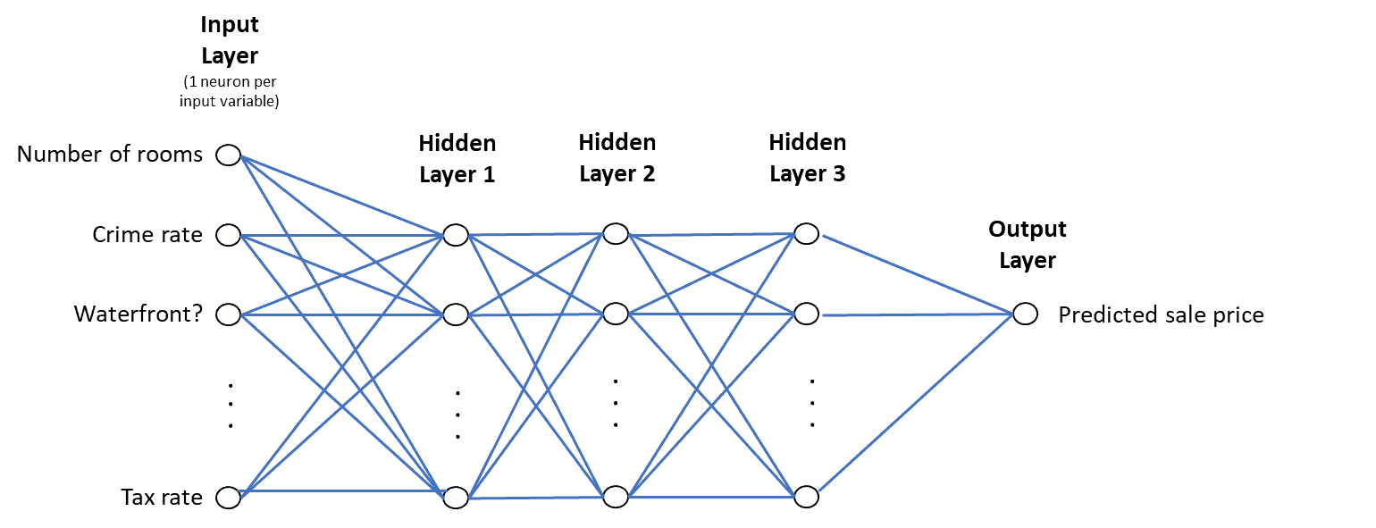
Below is an examples of a neural network with three hidden layers:

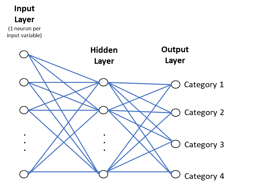
Here is an example of a neural network for a classification problem with four categories:

Some networks have fewer neurons in the hidden layers. These tend to be networks that are learning a reduced set of features possibly to be used as the pre-trained starting layers for another neural network (more on this below).

In general, neural networks with more layers and more neurons per layer can learn more complex functions. However, more layers and more neurons per layer also make a network more susceptible to overfitting especially if there are limited numbers of training examples. The number of layers and the number of neurons per layer are two of the more important hyperparameters that must be selected for neural networks.

3.3.7  Forward propagation

Here is what happens when we send a single training sample through the network: The system first multiplies each weight by the corresponding input variable, sums these together, and then applies an activation function (see below) to the sum to get the value of each neuron. The output layer is just one neuron which also has a set of weights, one weight for each neuron in the hidden layer. The computation for the output neuron is basically the same as for the hidden layer neurons except that the weights are applied to the hidden layer neurons instead of the input layer neurons. This process of propagating an input sample through a network is called forward propagation.

3.3.8  Backpropagation

The next step is to figure out how much to change each weight in the network to reduce the value of the cost function.

Earlier neural networks used a number of mostly trial-and-error means of adjusting the weights in the network to reduce the value of the cost function. In a landmark 1986 paper (Rumelhart et al, 1986), David Rumelhart, Geoffrey Hinton, and Ronald Williams showed that adjusting each weight by the partial derivative of the cost function with respect to that weight moves the cost function towards a minimum. It is called backpropagation because the partial derivatives are computed for the last hidden layer of the network and those values are used in calculating partial derivatives for earlier layers. So, the process works backward from the output to the first hidden layer. Each weight is adjusted by multiplying the weight by the partial derivative value and by the learning rate.

While the vast majority of deep learning networks use backpropagation, Hinton believes it is a dead-end method and has proposed a replacement known as the forward-forward algorithm (Hinton, 2022).  However, this algorithm doesn’t seem to be gaining traction in the year since it was proposed by Hinton.

3.3.9 Vanishing and exploding gradients

The goal of backpropagation is to update each weight in each neuron of each layer in a way that causes the predicted output to be closer to the correct output. The goal is to both minimize the error for each output neuron and for the network as a whole. Vanishing and exploding gradients (Glorot and Bengio, 2010) have been a significant issue for deeper networks.

3.3.9.1 Vanishing gradients

As just discussed, backpropagation starts with the weights on the links from the last hidden layer to the output layer. Because it’s not possible to directly compute the partial derivatives for weights in earlier layers, the computation used involves multiplying the partial derivatives from all later layers with the weights and values in the earlier layers. As a result, the earlier layers are susceptible to very small numbers that propagate backward. For example, when a neuron takes on the value of zero or one, the gradient becomes zero and that value propagates backward to all lower connected layers. If all the neurons in a given layer have a zero gradient, it propagates backward thereby killing any signal from flowing through these neurons. As a result, the network can fail to learn long-range dependencies (e.g. the dependencies of each word on other words in a sentence). The gradient is said to “vanish”.

3.3.9.2 Exploding gradients

Exploding gradients are the opposite of vanishing gradients. The multiplication during backpropagation causes bigger and bigger numbers until numerical overflows occur. Researchers have found ways of circumventing exploding/vanishing gradients:

• Lecun et al (1998) and Glorot and Bengio (2010) discussed the importance of normalizing the inputs so that the mean of each input variable is zero, the standard deviations of the input variables are roughly equal, and they are uncorrelated.
• The ReLU activation function (see below) and the GRU and LSTM neuron types (see below) are often effective in avoiding exploding and vanishing gradients.
• Batch Normalization (Ioffe and Szegedy, 2015) is also effective and commonly used.
• Dense convolutional networks (G. Huang et al, 2017) in which every layer is connected to every other layer in a feed-forward manner also appears to fix the problem.
• Gradient clipping (Pascanu et al, 2013) normalizes the gradients of a parameter vector when the sum of the least squares exceeds a threshold.

Other ways of avoiding these gradient issues will be discussed in the sections below on network architectures, activation functions and network tuning.

3.3.10  Batch vs stochastic gradient descent

Batch gradient descent (BGD) processes the whole dataset in each iteration of forward and backward propagation. This method can be very efficient if the entire dataset is small enough to do fit in memory with room for vector math in memory. More often than not, this isn’t the case and the dataset samples need to be split into mini-batches. This is called stochastic gradient descent (SGD). Because only a subset of the dataset is processed at any given time, the size of the subset can be chosen to fit in available memory. The most extreme form of SGD is where each mini-batch has just one sample. There are three primary advantages of SGD (LeCun et al, 1998):

• It is usually much faster than BGD and this is the primary advantage.
• Performance (e.g. accuracy) is often better.
• SGD can be used for tracking changes.

They also note the main advantage of BGD is that it is more likely to find a global minimum because it is less likely to get stuck in a local minimum. For SGD, single-sample mini-batches have advantages and some disadvantages. The advantages are:

• They produce a very noisy gradient that often switches directions. This can be helpful in pulling the process out of a local minimum.
• They require very little memory and will be much faster than using a mini-batch size that doesn’t fit in memory

The disadvantages are:

• It can take a long time to converge
• It can be so noisy that it pulls the process out of the global minimum

In practice, batch and single-sample SGD are rarely used and the most common mini-batch sizes range from 50 to 256 samples for neural networks. In Keras, the mini-batch size is controlled by the batch_size parameter to the layer constructor (in the code example above, batch_size is an optional parameter to the Dense constructor).

3.3.11 Momentum methods

One problem with stochastic gradient descent is that it has difficulty in regions where one dimension slopes up and another slopes down (e.g. Dauphin et al, 2014).

A momentum parameter is used that is analogous to the friction that occurs when a ball rolls down the hill. The friction will be reduced and the velocity increased when the dimensions slope in the same direction and friction will be increased and velocity reduced when they don’t.

Some implementations use a constant value (.9). Some start with a smaller value (e.g. .5) and increase over multiple epochs to .99. Nesterov momentum is a variant that has been shown to increase the performance of recurrent neural networks on a number of tasks (Bengio et al, 2012).

In the Keras example above, the SGD optimizer is specified in the .add method (‘sgd’). Keras offers a large number of optimizer choices including RMSprop, Adagrad, Adadelta, Adam, Adamax, and Nadam, any of the TensorFlow optimizers, and the ability to code your own optimizer. For an analysis of which optimizers work best for which tasks see Schmidt et al, 2020.

The Adam optimizer is probably the most widely used as of early 2023.

3.3.12 Learning rate optimization

As discussed in the previous section, a learning rate that is too small will take forever to converge and a learning rate that is too high will keep over- and under-shooting the minimum. Annealing is a technique that reduces the learning rate when progress slows below a threshold. In many tools, one can either set a fixed learning rate or use a callback to define a function that adjusts the learning rate based on the progress. There are also a number of SGD variants that change the learning rate dynamically. These methods are particularly effective if the data is sparse (for example, sparse data might result from using one-hot encoding of lots of categorical variables) and include:

RMSprop: Divides the gradient by a running average of the gradients over time that is weighted towards more recent gradients. This is a good choice for RNN networks.

Adadelta: Keeps an average of the squares of the gradients over time that is weighted towards more recent gradients and automatically changes the learning rate. Most importantly, it changes the learning rate for each parameter rather than applying the same learning rate for each parameter. For sparse data, it will use a faster learning rate for parameters that are infrequently updated (Zeiler, 2012).

Adam: Similar to Adadelta, Adam keeps an average of the squares of the gradients and changes the learning rate for each parameter but also keeps an average of the gradients themselves and is, therefore, a cross between Adadelta and a momentum algorithm.

Nadam: Combines Adam and Nesterov Momentum

Other optimizers in this category include Adagrad and Adamax. In Keras, each optimizer has a learning rate parameter. Some optimizers such as SGD have additional parameters. For SGD, one parameter is whether or not to use the Nesterov Momentum version of SGD.

The Adam optimizer has become the most commonly used optimizer.

3.3.13  Activation functions

3.3.13.1 Hidden layer activation functions

Each neuron in each hidden layer receives input from one or more neurons in a previous layer and each input has a weight. For example, the neurons in the first hidden layer receive inputs from the neurons in the input layer. To compute the value of a neuron in a hidden layer, one sums the values of each incoming neuron multiplied by its weight. Then the sum is passed through an activation function. The purpose of an activation function is to improve the ability of the network to capture non-linear relationships. In the earliest neural networks, the activation function was typically a simple step function, i.e. if the sum of the weighted values was greater than or equal to a threshold (e.g. .5), the neuron value would be 1 and 0 if less than .5. Three of the most commonly used activation functions for hidden layers are:

Sigmoid: The sigmoid function compresses values into a range of 0 to 1 in an S-shaped curve. It was popular up until a few years ago but rarely used today because of the vanishing gradient problem. Another issue with sigmoid activation is that its outputs are not zero-centered. This causes zig-zagging in the gradient descent.

Tanh: The hyperbolic tangent function compresses values into a range of -1 to 1. It has a similar shape to sigmoid function but its outputs are zero-centered. This activation is still widely used for networks with a single hidden layer and for tasks other than image processing and natural language processing.

ReLU: Rectified linear units (ReLUs) set the value of the neuron to 0 if the input value is less than and to the value itself if the input value is greater than 0 (Glorot et al 2011b). This results in a lot of zero-valued neurons (i.e. a sparse network) which leaves the non-zero neurons with strong signals that tend to avoid vanishing gradients. ReLU accelerates the convergence of gradient descent by six times vs. the sigmoid and tanh functions (Krizhevsky et al, 2012).

It is computationally inexpensive because there are no exponents to compute (unlike tanh). When using ReLU activation, one has to be careful not to set the learning rate too high because it can cause neurons to “die”. ReLU is usually the choice for image processing tasks and is also commonly used in natural language processing tasks. There are also a number of ReLU variants in use such as Leaky ReLUs (Maas et al, 2013) and PReLUs (He et al, 2015a). Glorot et al (2011b) showed that training is much faster if ReLU activation is used in a deep learning network. In the Keras example above, the ReLU activation function is specified. Keras supports many other activation functions including softmax, elu, selu, softplus, softsign, tanh, sigmoid, hard_linear, PReLU, LeakyReLU, and the ability to code your own optimizer.

3.3.13.2 Output neurons

Output neurons work basically the same way as input neurons but have specialized activation functions. For example, a regression problem with a quantitative output will usually have a single output neuron and the output value will simply be the sum of the weighted inputs (i.e. no activation function). A yes/no (binary classification) problem will also have a single output neuron and will use a sigmoid activation to map the value to the 0 to 1 range. A post-processing function then outputs ‘yes’ if the value is >=.5 and ‘no’ otherwise. For multi-category classification, there is one neuron per category, and a softmax activation function is typically used. The softmax function will create a probability of each classification with the sum of the probabilities summing to 1. The highest probability classification is selected.

3.3.14  Reducing overfitting

Regularizers reduce overfitting by helping keep weights and/or layer outputs from getting too large. L2 regularizers add additional terms to the cost function that penalize large values.

L1 regularizers add terms that cause weight vectors to become sparse. Regularization terms can also be added to layers in a neural network. In Keras, regularizers are specified as optional parameters to the layer initialization function. L1, L2, and ElasticNet regularizers are provided and custom regularizers can be coded.

L2 regularizers add the square of the sizes of all the weights so that the system “prefers” evenly-distributed weights over a small number of large weights. L1 adds a term that encourages the focus on a small subset of input neurons to eliminate “noise”. The use of L2 regularization combined with dropout layers is a common practice for avoiding overfitting. Arpit et al (2017) showed that regularizers can prevent networks from simply memorizing the data even where they have enough capacity to memorize.

The downside of regularizers is that, while they improve overall performance, they result in improvement in some classes at the expense of decreased performance in other classes (Balestriero et al, 2022).

Dropout layers randomly set a subset of the neuron outputs from the preceding layer to 0 for each training iteration. This prevents neurons from developing too many co-dependencies with other neurons (Srivastava et al, 2014) and forces network to create redundant connections.

This essentially forces the network to learn features that only depend on the activation of a single neuron and don’t require other neurons to be active. The effect is almost like sampling from many different networks. This helps reduce overfitting as it causes different neurons to be active for different parts of the dataset.

The percentage of neurons to be dropped is a parameter that must be tuned – often by trial-and-error. If the parameter is too small, it won’t have the desired effect. If it is too large, the performance of the network will be reduced considerably. Srivastava et al recommend dropping between 20% and 50% of the neurons in each dropout layer.

Batch normalization (Ioffe and Szegedy, 2015) normalizes layer inputs for the next layer (converts them to zero mean and unit variance – more on this later).  The goal is to reduce the effects of covariate shift.  Covariate shift refers to input data that was collected over time and in which the distribution of independent variables has changed over time. It also reduces the impact of the initial values and the scale of the parameters on the gradient computations. 

Batch normalization speeds up training for convolutional neural networks (see below) and other fully-connected neural networks but doesn’t work well with recurrent neural networks (see below). See this blog post for a good explanation of how batch normalization works.

Layer normalization (Ba et al, 2016) is similar to batch normalization but it adjusts the mean and variance as the neuron values in a layer are being computed.  Unlike batch normalization, it works well for recurrent neural networks and transformers.

3.3.15 Performance and model complexity

Before the advent of neural networks, conventional wisdom held that increasing the number of parameters in a machine learning model helped performance up to a point. After that point, increasing the number of parameters resulted in overfitting. In other words, adding parameters would improve training performance but decrease test performance.

Neural networks show that same pattern. After some number of parameters, test dataset performance decreases.

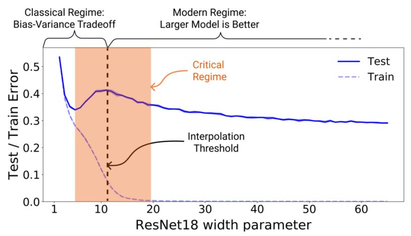
This is thought to be a result of overfitting.  However, for some models, as the number of parameters increases even further, test performance actually improves considerably (Nakkiran et al, 2019), a phenomenon known as double descent. Test performance continues to improve even after the point at which the complexity of the network is high enough to learn even the random patterns in the training data.

A similar result was observed by OpenAI researchers (Powell et al, 2022) that they termed grokking.  It is illustrated below:

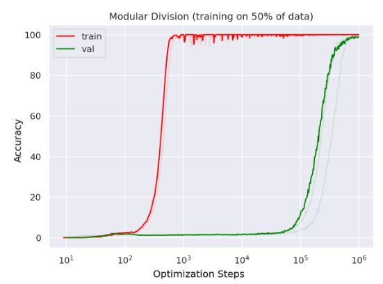
Because the system quickly achieve near perfect accuracy on the training set while seeing zero accuracy on the test set, researchers conclude that the training set is being memorized and that there is no generalization occurring.  However, over time, accuracy on the test set starts to increase which is evidence that generalization is occurring.

MIT researchers Frankle and Carbin (2019) found a way to reduce network complexity without reducing performance or requiring longer training times. They postulated that there will usually be a sub-network that is a small fraction of the size of the full network and that can be trained in the same number of iterations to produce equivalent performance.

This is known as the Lottery Ticket Hypothesis. To find the optimal sub-network, they train a network and then discard connections and neurons with small weights. Then they start over and train the network from scratch and again throw out connections with small weights and repeat the process.

On two different image processing tasks, they were able to find a sub-network that was 10-20% of the size of the full network and achieved comparable performance to the full network.  Another group of MIT Researchers (Lai et al, 2021) were able to obtain a similar result for speech recognition.

Other methods for reducing model size without impacting performance can be found in a Google Research paper (Menghani, 2021).

3.3.16 Performance and dataset size

Historically, the rule of thumb for data scientists was that more data is always better. The rule of thumb for neural networks was that a supervised learning network would achieve acceptable performance with around 5,000 labeled observations per category (Goodfellow et al, 2016).

More recently, researchers have found the double descent phenomenon also occurs in the relationship between the number of observations and test performance (Nakkiran et al, 2019).

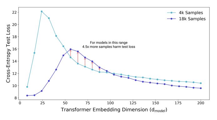
Image source:  Nakkiran et al, 2019

Just as for model complexity, neural networks have turned this relationship on its ear. For neural networks, test performance improves as the number of observations increases up to a point. After that point, more observations decrease test performance. But again, that only happens up to another point after which test performance again starts improving.

3.3.17 Performance, computing power, and training time

Researchers have also studied test performance as a function of computing power and, not surprisingly, found that performance is directly correlated to computing power (Thompson et al, 2020). This result is not surprising because increased computing power enables more complex models and the processing of larger datasets. However, training huge models requires a massive computing infrastructure that is available to relatively few researchers.

Microsoft researchers (Ren et al, 2021) developed ZERO-OFFLOAD, an architecture that enables moving much of the processing off of the GPU(s) and onto the compute and memory functions of a computer. This enables training of massive models on machines with even a single GPU without requiring changes to the underlying model architecture.

Researchers are also working on ways of reducing the computational requirements of specific model architectures. For example, Nvidia researchers (Mandava et al, 20201) have developed a methodology for reducing the compute time of transformer architectures by 35%.

Other researchers (Choromanski et al, 2021) have shown how to reduce both the space and time requirements of transformers from quadratic time to linear time. Munich researchers (Schick et al, 2021) have replicated the capabilities of the massive GPT-3 system that has 175 billion parameters with a system that has “only” 223 million parameters (i.e. 0.1% of the parameters in GPT-3). Similarly, Google researchers (Kaliamoorthi et al, 2019) have developed an architecture that replicates the capabilities of the BERT system (110 million parameters) with an architecture that contains only 200 thousand parameters).

3.3.18  Memorization

Neural networks sometimes memorize the relationships between input and output variables. Zhang et al (2017) created a network that could learn to classify images with relatively little generalization error (i.e. the test error increased very little vs. the training error). Then they tried feeding the same untrained network images whose labels were randomized (e.g. a cat might be labeled ‘dog’ and another cat might be labeled ‘fish’). Intuitively, one would expect little or no learning to occur and a training error that would be at the level expected for random guessing. Surprisingly, the network converged with a training error near zero. Not surprisingly, the test error was huge and at the level expected for random guessing.

What had happened was that the network memorized the training examples. Of course, since it had learned a random set of labels, there was no generalization. This was a demonstration of near 100% overfitting.

Berkeley researchers (Carlini et al, 2021) showed that it was possible to extract personal information that had been memorized by a large neural network.  This data included names, phone numbers, email addresses, chat conversations, and UUIDs. 

A Google researcher (Feldman, 2021) wrote a paper that was aptly titled “A short tale about a long tail”.  His study showed that, for both images and text, networks tend to memorize labels for less frequently occurring data (i.e. the long tail of the data distribution).

In another article, Berkeley researchers (Wallace et al, 2020) found evidence of memorized content in GPT-2 such as news headlines, Donald Trump speeches, pieces of software logs, entire software licenses, snippets of source code, passages from the Bible and Quran, and the first 800 digits of pi. Subsequent research (Arpit et al, 2017) has shown that deep learning networks learn patterns of data, if they exist, before they resort to memorization. However, memorization of at least some training observations always has to be considered as a possible explanation of deep learning results. Memorization can also occur as a result of faulty training methodologies that cause data leakage.

See also the discussion of memorization in large language models.

3.3.19 Overfitting

Memorization is one factor that can result in overfitting and poor generalization to test data and the real world.  Simon et al, (2021) developed a set of principles that appear to explain why some optimization algorithms and hyperparameters result in good generalization to test and real-world data while others do fine on the training data but result in poor generalization.

3.4  Convolutional neural networks

Convolutional Neural Networks (CNNs) have had tremendous success in image processing tasks such as handwriting recognition and finding and classification objects in images. CNNs were inspired by the work of two Harvard Medical School researchers who found that stimulating small regions of the visual field result in the firing of a single neuron in the brain of a cat.

The initial major success for CNNs took place in 1997 when Yann LeCun and colleagues at Bell Labs created a CNN that was used commercially to read the handwritten letters and numbers written on checks (LeCun et al, 1997). In the simple neural networks discussed above, every node in a layer is connected to every node in the next layer. In a CNN, that is not the case. The connections are sparse (meaning only some layers are connected to other layers) leading to higher computational efficiency.

3.4.1 Input layer

The input layer will typically be a 3-dimensional array. For example, an image with 640 pixels of height and width and 3 RGB (Red, Green, Blue) values will be a 640 x 640 x 3 array. Each element of the array might have a value between 1 and 128 representing the intensity of the red, green, or blue color. For simpler images like handwriting samples which are just black and white, a typical array size is 28 x 28 x 1.

3.4.2 Convolution layer

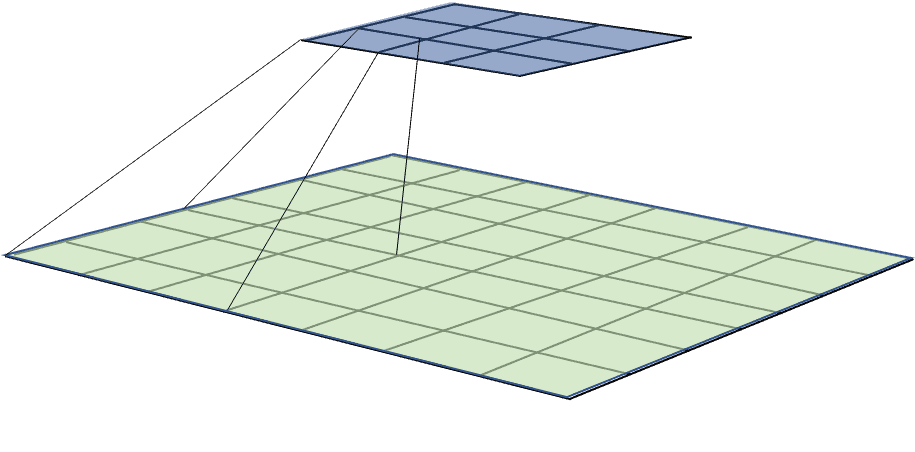
CNNs use feature maps and pooling layers for image analysis. The mathematical name for the filtering operation performed by a feature map is a convolution. These pooling layers provide invariance to translation, rotation, and scaling. In CNN-based image processing tasks, the input layer neurons (variables) are typically the pixels of an image.  The figure below show a mapping in a CNN from the input layer to the first hidden layer. In this figure, we map from a 7×7 layer to a 3×3 layer:

To explain how this works, let’s use an even simpler example of an input image of the number ‘7’ with pixels on the left and values on the right:

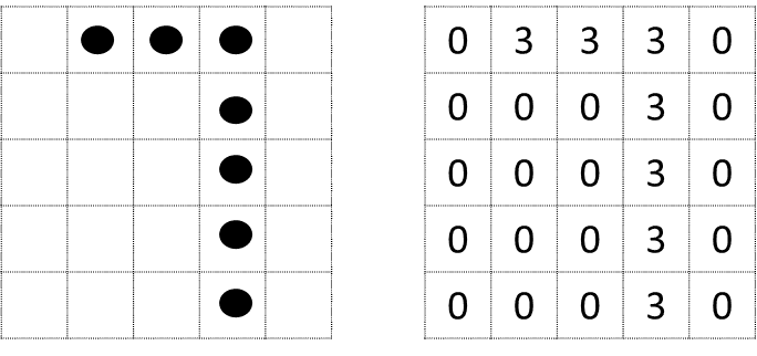
Suppose our input images are 5x5x1 pixels (i.e. grayscale) as shown in the left side of the figure above. In reality, these images would be too small to hold anything of interest but they will be used here for purposes of illustration. And let’s suppose that each cell in the array had a value of 0 to 3 where 0 is no gray (white) and 3 is black. On the right side is the image represented as an array of its numeric pixel intensities. Next we’re going to define a filter that we’re going to superimpose on various areas of the image:

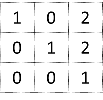
This filter is 3×3. The first step is to superimpose the 3×3 filter on the top left of the image. Then, we’re going to multiply the value of each cell in the filter by the value of the image pixel it is superimposed over, sum the results, and put the sum in the top-left cell of a new matrix. Then we’ll shift the filter over by 2 and repeat the process. At this point, we’re over the top-right cells and we repeat the process. Then we’ll go back to the left but shift the filter down by 2 cells and continue on until the filter is over the lower right cells of the image.

The end result will be a new 2 x 2 matrix shown below:

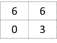
Two issues that need to be mentioned with this new 2 x 2 matrix are that we’ve now downsized from 5 x 5 to 2 x 2. First, it’s been shown that downsizing too fast is problematic. Also, the information at the edges isn’t well-represented. To fix these two problems, it is common to zero-pad the original image. For example, if we were to add two rows and two columns of zero-padding, we would end up with a 4 x 4 matrix. This resultant matrix is known as a convolution. So, now we’ve defined a filter that has three properties:

Kernel size (e.g. 3 x 3).

Stride. A stride of 2 means shift the filter right by 2 pixels to compute the second neuron in the first row of the hidden layer. Shift by one more to compute the third neuron and so on. After the first row of the hidden layer is computed, shift the filter all the way back to the left and move down one row and continue the process.

Padding. The additional rows and columns of zeroes of input neurons.

A typical CNN uses multiple filters with different values to find different features in the images. Each different filter creates a different filter map.

3.4.3  Pooling layer

After a convolution layer, you will most often see a pooling layer. Pooling is also known as down-sampling and/or sub-sampling. A pooling layer also has a sliding window but the filter works differently than in a convolution layer.

First, the stride is chosen so that the filter windows do not overlap the way they can in a convolution layer.

Second, instead of a filter where the filter values are multiplied by the previous layer outputs, a pooling layer just takes the maximum value. While max poolingis the most common, one can also take the average or some other function. With L2 pooling, one takes the square root of sum of the squares of the values in the window.

Applying a filter in the convolution layer to multiple contiguous areas results in features detected that are translation invariant (i.e. it won’t matter where in the image the feature occurs). Pooling tells the system whether or not the feature was found anywhere in the image. Pooling also reduces computation by eliminating non-maximal values and reduces computation further by reducing the number of parameters that need to be estimated.

For example, a 2×2 pooling filter will reduce the dimensionality by a factor of 4 which reduces the number of parameters that must be estimated by a factor of 4. The above description might sound a little intimidating but the code for CNNs can be quite simple. The example below uses the MNIST database of 60,000 handwritten digits:

The code below creates a CNN that is somewhat similar to the LeCun et al (1998) network named LeNet-5 but uses a lot more feature maps to take advantage of the easy availability of processing power today versus 20 years ago. The average pooling layers are slightly more complex than usual: each neuron computes the mean of its inputs, then multiplies the result by a learnable coefficient (one per map) and adds a learnable bias term (again, one per map), then finally applies the activation function. Most neurons in C3 maps are connected to neurons in only three or four S2 maps (instead of all six S2 maps).

The code above show a sample CNN. It creates an initial convolution using 32 5×5 filters resulting in 32 feature maps (LeNet-5 used 6 feature maps). A stride of 1 is used to keep the output layer only a little smaller (24×24) than the input. A max-pooling layer is next with a filter size of 2×2 and a stride of 2×2 reducing the output size by a factor of 4. Then another convolutional layer this time with 64 5×5 filters followed by another max-pooling layer. Then there is a Flatten layer to flatten out the convolutions so they can be input to a Dense (fully-connected) layer with 1000 neurons which is large enough to contain most of the information in the last pooling layer. And finally that layer is connected to another Dense layer with only 10 neurons – one for each category. The neuron with the highest value is the choice for the input image.

3.4.4  Feature learning

It is generally thought that the initial layers of CNNs learn low-level features such as edges, lines, and curves (Zeiler and Fergus, 2014). A visualization of features learned by a CNN is shown below:

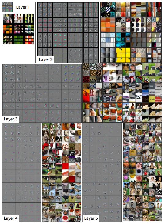
Features extracted in Layer 1 appear to be very simple features.

In Layer 2, we start to see edges and color gradients.

In Layer 3, there are textures such as mesh patterns.

In Layer 4, we start to see class-specific features such as dog faces and bird legs.

In Layer 5, we see entire objects such as dogs and keyboards. Quoc Le and his colleagues (2012) trained a network on 10 million high-quality (200 x 200) images using an autoencoder. They then examined all the neurons in later layers to find which neuron was the best predictor of a human face. That neuron by itself was able to correctly determine if an image was a human face 81.7% of the time in the test set of images. They were able to get a similar result for recognition of human bodies and cats. So, for a facial recognition network, the higher-level features might include a detector like Le’s that can determine whether it’s a human face or not. There might also be specialized detectors for eyes and noses. Higher up there might be specialized features to detect the face of a specific person.

3.4.5 CNN applications

CNNs have been mostly used in computer vision applications such as image classification, facial recognition, pedestrian recognition, and handwriting recognition. However, they are also used in many other areas such as gene phenotyping (Ning et al, 2005), detection of diabetic retinopathy (Gulshan et al, 2016), detecting cancer metastases (Y. Liu et al, 2017), and speech recognition (e.g. Hinton et al, 2012).

3.4.6  CNN improvements

The UNet architecture (Ronneberger et al, 2015) is an improvement on the CNN architecture in which a series of upsampling layers is added to the downsampling layers.  U-Nets have achieved widespread use in image generation foundation models including DALL•E 2 and Stable Diffusion.

Researchers have created many other advanced architectures that improve on the basic CNN idea such as capsule networks (Sabour et al, 2018; Punjabi et al, 2020) and EfficientNet (Tan and Le, 2020).

3.5  Recurrent neural networks

When you read a sentence that starts The shooter fired a … you expect the next word to be “bullet”. This expectation becomes a possibility when you read the word “shooter” and becomes a strong probability after encountering the word “shooter” and an even stronger one after encountering the word “a”. To create this building expectation, all three words are required. For a neural network to do this, some form of memory is required for the sequence of words. Recurrent neural networks (RNNs) provide a form of memory and differ from the networks discussed to this point in two significant ways:

1. Loops. The neural networks discussed to this point (including CNNs) are feedforward only, that is the output from one layer feeds forward to the input in the next layer. There are no loops. RNN networks have loops. Each neuron’s last output is saved and is fed back into the neuron as an input. Therefore, each neuron has double the input weights – one for the regular connection and one for the memory of the previous output. The cost function is designed to to minimize both sets of weights. The previous output essentially provides a form of ‘memory’.
2. Sequences. The networks discussed to this point all have fixed length inputs and fixed-length outputs. For example, in image classification, the inputs are images with a fixed number of pixels and the output is a classification with a fixed number of categories. RNN networks are often the right choice when the inputs and/or outputs are variable-length sequences. Some examples of tasks that can be formulated as sequence tasks include:

• • Image captioning (adding captions to images) is an example of a fixed-length input (images with a fixed number of pixels) to a sequence output (words or characters of variable length).
  • Sentiment analysis has sequence input and categorical output.
  • Machine translation, question answering, speech recognition, text to speech, video captioning all have both variable-length inputs and outputs. These are known as sequence-to-sequence tasks (see below).

One simple method for dealing with variable length sequences is to map the variable-length sequences into a fixed-length sequence that is the maximum length and fill it will nulls.

RNN’s have proven to be extremely powerful. RNNs have achieved state of the art performance in tasks such as machine translation and automated speech recognition. RNNs can even be fed a large text (or handwriting) sample and generate text (or handwriting) in the same style.

For example, Sutskever et al (2011) trained RNNs on Wikipedia, the New York Times, and some academic papers. In each case, the RNN produced text in the style of the input. To be clear, the text produced wasn’t completely grammatically correct or at all lucid but at first glance is recognizable as text of the input style.

Graves (2014) did the same for Wikipedia and cursive handwriting.

Andrej Karpathy, the Director of AI at Tesla, wrote a great blog post on the surprising power of RNNs. He trained character-to-character networks on War and Peace, Shakespeare, and other texts. The examples in his blog are illustrative of both the power of RNNs and perhaps also the limitations. Moreover, in the War and Peace examples, he shows how the system learns over time with more and more iterations of training data. For example, after 100 iterations, the system starts to get an idea of words separated by spaces:

tyntd-iafhatawiaoihrdemot lytdws e ,tfti, astai f ogoh eoase rrranbyne ‘nhthnee e plia tklrgd t o idoe ns,smtt h ne etie h,hregtrs nigtike,aoaenns lng

At 300 iterations the model starts to get an idea about quotes and periods:

Tmont thithey” fomesscerliund Keushey. Thom here sheulke, anmerenith ol sivh I lalterthend Bleipile shuwy fil on aseterlome coaniogennc Phe lism thond hon at. MeiDimorotion in ther thize.

At iteration 500 the model has now learned to spell the shortest and most common words such as “we”, “He”, “His”, “Which”, “and”, etc.

we counter. He stutn co des. His stanted out one ofler that concossions and was to gearang reay Jotrets and with fre colt otf paitt thin wall. Which das stimn

At iteration 700 more and more English-like text emerges:

Aftair fall unsuch that the hall for Prince Velzonski’s that me of her hearly, and behs to so arwage fiving were to it beloge, pavu say falling misfort how, and Gogition is so overelical and ofter.

At iteration 1200 one can see use of quotations and question/exclamation marks. Longer words have now been learned as well:

“Kite vouch!” he repeated by her door. “But I would be done and quarts, feeling, then, son is people….”

At iteration 2000, the system starts to properly spell words and names, and use quotations properly:

“Why do what that day,” replied Natasha, and wishing to himself the fact the princess, Princess Mary was easier, fed in had oftened him. Pierre aking his soul came to the packs and drove up his father-in-law women.

These examples make one wonder what would happen if we fed in enough data and used enough iterations. For example, if we fed in everything Shakespeare had written, would we eventually get new plays and sonnets that read as if Shakespeare had written them posthumously? If we fed in all of the speeches of president of the United States, would the presidents no longer need human speech writers? Certainly not. One reason is that the knowledge about current human events required to write presidential speeches just isn’t contained in speeches about past human events.

3.5.1  Long short term memory networks

RNNs are fairly good at capturing short-term dependencies. Suppose, for example, that we are using an RNN to predict the next word in a sequence. The next word in this sequence is obvious:

The shooter fired a …

Here it is clear the next word will be bullet and an RNN would likely have little difficulty making this connection. However, the next word in this sequence is not so obvious:

John hit the …

We don’t know if it’s “ball”, “car”, “wall” or one of many other possibilities. However, an RNN might have trouble when the distance between the sequence is:

John was playing baseball with his friends.

It was John’s turn to hit.

John hit the …

It’s obvious to people that the next word is most likely “ball”. An RNN would like have difficulty making the connection between “baseball” and “ball” because of the number of words that had been processed since the word “baseball” had been encountered. This is known as a long-term dependency. RNNs have trouble with long-term dependencies.

Long short term Memory (LSTM) networks, first proposed by Hochreiter and Schmidhuber (1997) are a special type of RNN network designed to help with long-term dependencies by providing a long-term memory capability. In a vanilla RNN network, the hidden state of the neuron and the output of the neuron are the same. In an LSTM neuron, they are different. Each LSTM neuron has 3 gates, each with its own weight:

• The weight on the input gate that determines how much of the current input to remember
• The weight on the forget gate that determines how much of the previous input to forget
• The weight on the output gate determines how much of the internal state to pass on to the next time step and any higher layers

LSTM’s essentially function as an internal memory that is different from what is passed on to the next time step and any higher layers. LSTM networks are especially useful for text processing tasks like machine translation and speech recognition.

3.5.2  Gated recurrent units

A Gated Recurrent Unit (GRU)(Cho et al, 2014) neuron is a simpler variant of an LSTM neuron that often performs equally well but is computationally more efficient. Unlike an LSTM, a GRU neuron has no output gate. It only has input and forget gates so the entire state is passed on to the next time step and higher layers. Like LSTM networks, GRU networks are often used in text processing tasks.   See this blog post for a good explanation of LSTM’s and GRU’s.

3.5.3  Bidirectional RNNs and LSTMs

In a bidirectional RNN, two RNNs are trained in parallel. The first takes the input words in the normal (forward) direction. The second takes the input words in the reverse direction, starting from the last word. The outputs are then combined via concatenation (or multiplication, addition, or averaging). This scheme has been found to improve performance in tasks where the prediction of a word or character is dependent on both the words preceding and the words following. A bidirectional LSTM is conceptually the same; however, LSTMs are used instead of vanilla RNNs.

3.5.4  Issues with long-term dependencies

RNNs have some memory for their prior states. However, Bell Labs researchers discovered back in 1994 (Bengio et al, 1994) that RNNs have difficulty with long-term dependencies. To use an example from a Google blog (Uszkoreit, 2017), consider the sentence

I arrived at the bank after crossing the road

I arrived at the bank after crossing the river

The meaning of the word “bank” will depend on whether the next word (the disambiguating word) is “road” or “river”. An RNN has a difficult time because it must choose the appropriate word sense before it encounters the disambiguating word. By the time, the word “road” or “river” is encountered, the word “bank” has been forgotten and replaced by a set of weights.

It has been known for over 20 years (Bengio et al, 1994; Hochreiter et al, 2001) that the more time steps (e.g. words) between the ambiguous word and the disambiguator, the poorer the outcome because the system forgets earlier words in a sentence as it processes the later words in the sentence.

LSTM’s and bidirectional networks do better with long-term dependencies than plain vanilla RNNs but even these architectures still have issues with long-term dependencies.

Google’s DeepMind unit proposed its Differentiable Neural Computer (DNC) architecture as a possible solution to this issue (Graves et al, 2016).  The DNC architecture is analogous to a computer architecture that has a CPU controller and a memory.  The DNC has one network that acts as a controller that takes inputs, performs inference, and produces outputs for various tasks such as question answering.  A second network maintain a memory of past activations of the network for past questions.  The controller network can access this memory during the inference process to create answers. However, attention architectures, which will be discussed shortly, provide a much better solution for long-term dependencies.

3.6  Sequence-to-sequence learning

Two papers written in 2014 put sequence-to-sequence (seq2seq) learning on the map and set the stage for machine translation to quickly move from so-so translations to remarkably good translations. 

The first paper (Cho et al, 2014) proposed a new type of network known as an encoder-decoder network that is composed of two GRU-based RNN networks below:

During training, the first network, termed the encoder, maps the source language sentences into an internal representation.

The second network, termed the decoder, maps the internal representation into a target language sentence. More specifically, the decoder is trained to predict the next word in the target language sentence given the internal representation plus the already-translated words in the target sentence.

Importantly, the two networks are trained at the same time using a single cost function based on the difference between the system’s translation and the correct translation. The network essentially learns a distribution that can predict the first word and each next word in the target language.

In fact, the Cho et al system was not used to directly translate text. Instead, the learned distribution was used to re-score and improve the translation selections made by an earlier machine translation technology known as phrase-based machine technology which is discussed in the machine translation chapter.

Google researchers (Sutskever et al, 2014) developed an encoder-decoder architecture that produced nearly-equivalent performance to the best phrase-based machine translation systems at the time.  In their architecture, both the encoder and decoder were LSTMs. Their primary innovation over the Cho et al architecture was to reverse the order of words in the input. This helped with the long-term dependencies. In the “bank” example above, the context word “river” is encountered before the word that needed disambiguation (“bank”).
The encoder-decoder architecture by itself had one major limitation: All of the information about the source language sentence and how to translate it into the target language had to be shoehorned into the final hidden state of the encoder and that was the only information the decoder could use.

One problem with this approach is that the internal representation produced by the encoder is most influenced by the last word in the sentence and least influenced by previous words. By the time the last word in a long sentence is encountered, the encoder might have completely “forgotten” the first word.

Another problem is that some information present in the earlier hidden layers is almost certainly lost by the process of shoehorning all that information into the final layer.

One final improvement that was needed to vault neural machine translation systems into the lead position in the machine translation field was the attention mechanism developed by Google researchers (Bahdanau et al, 2015) illustrated below:

The Google attention mechanism is a simple feed-forward neural network that uses the representations from all time steps of the input sequence to build a detailed relationship between the input words and the output words.  Below is a different illustration of the encoder-decoder with attention architecture:

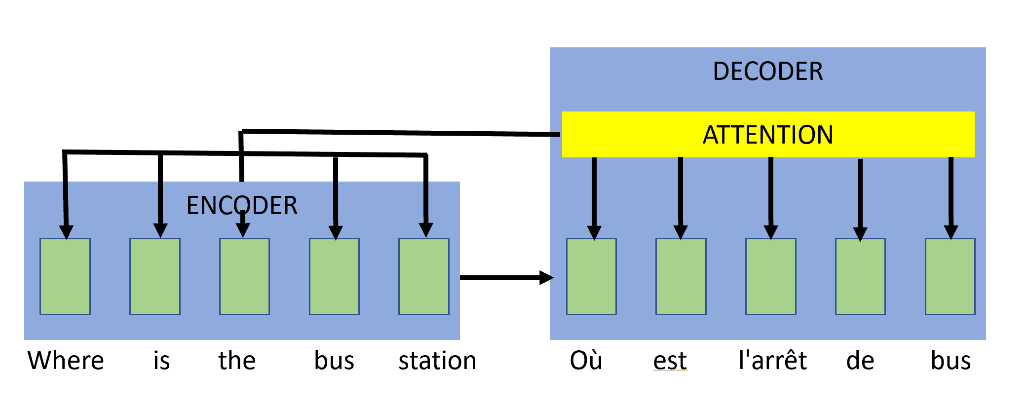
In a machine translation task, it learns how words affect each other with respect to machine translation. Specifically, it learns how other words might contribute to disambiguation and/or to many-to-one or one-to-many mappings from a word in the source language to a word in the target language. It gives the decoder access not only to the final hidden layer but to the information in the hidden layers corresponding to each time step (i.e. word) in the source sentence.

The primary job of the attention mechanism is to learn how words and phrases from the source language align to the target language as illustrated below:

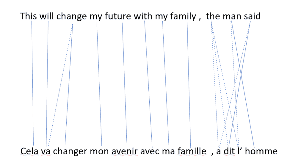
The lines in the diagram show what the system learned with respect to which words to pay attention to as it generates the next French word. It has learned that “man” in English contributes to the translations of three words in French: “l’”, and “homme”. The word “the” contributes to the translation of three words in this sentence and the system probably learns that the word “the” contributes in other ways in other English sentences. It learns that to translate this sentence, attention must be paid to both “the” and “man” in order to select the correct “l’” and not the incorrect “le”, “la”, or “les”. Only by also considering “man” was it able to make the correct choice.  

3.7 Transformer networks

In 2017, a team of Google researchers (Vaswani et al, 2017) published a paper that was cleverly-named “Attention Is All You Need” in which they describe their transformer model which has become the go-to architecture for many current natural language processing systems. The transformer architecture has three improvements over the Bahdanau et al encoder-decoder plus attention model. First, the encoder and decoder models each include a self-attention network in addition to an attention network that looks at both the input and output word sequences as illustrated below:

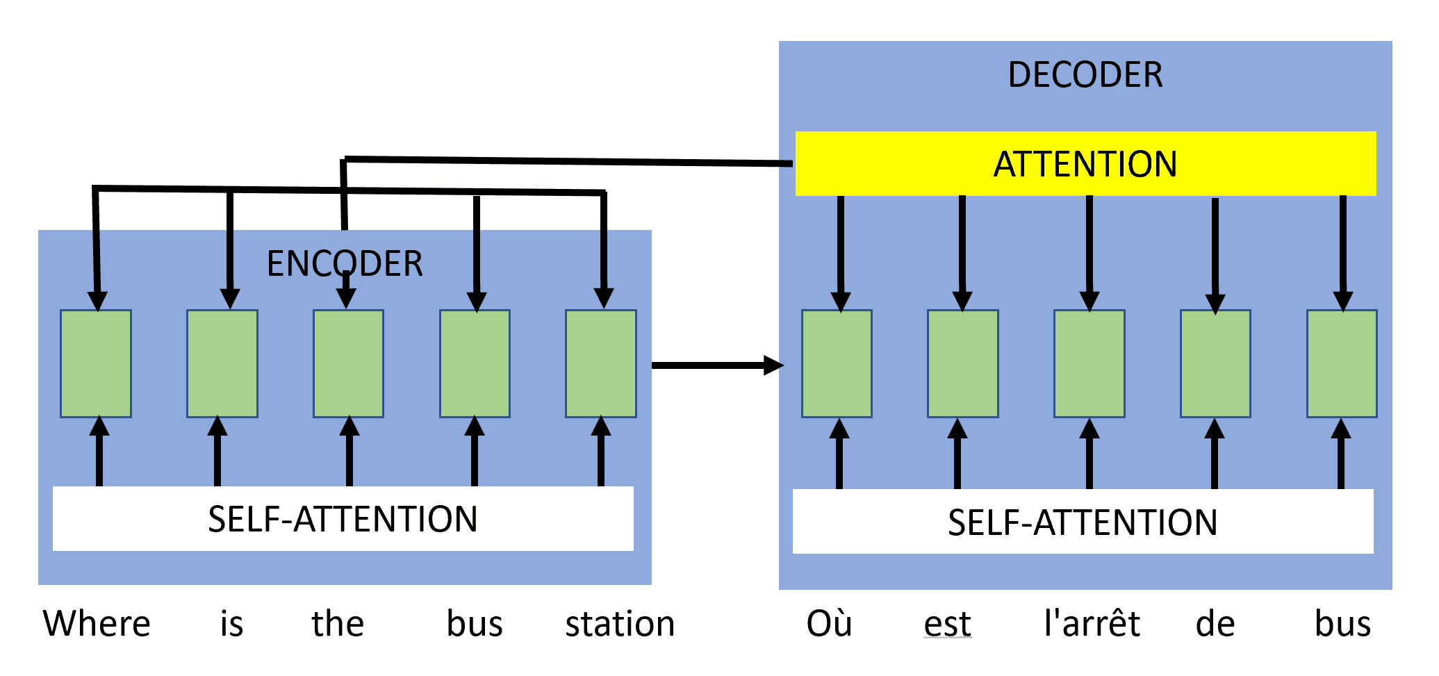
Rather than processing the input left to right as happens in a plain vanilla encoder-decoder model, the attention mechanism makes it possible for the network to “pay attention” to all the words in the input and output at all times.  The attention mechanism learns which words are most important for machine translation task.  In other contexts, such as question answering, the attention mechanism might learn that other words are more important.

Compared to LSTMs, attention mechanisms have two advantages:  First, they have no recency bias.  Second, they are learnable as opposed to hard-wired.

A transformer attention mechanism captures dependencies between the source and target language words such as disambiguation dependencies. When attention is used within an input sequence, it is known as self-attention. The transformer architecture also provides self-attention to the target words generated by the decoder.

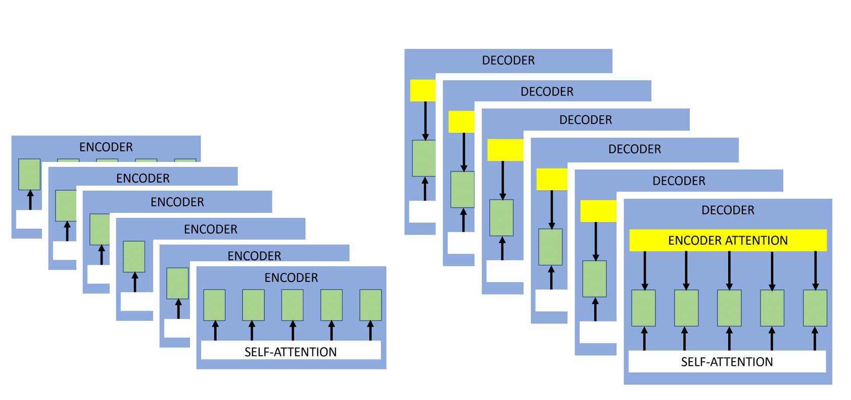
The transformer architecture also uses multiple encoders and decoders. In the original Vaswami et al paper, six encoders and six decoders were used.  Each encoder-decoder pair is known as a head.  The use of multiple heads allows for the model to learn different types of relationships and dependencies within a sequence.  Their outputs are then combined to form a final representation.

This architecture turned out to be so powerful that it obviated the need for use of a recurrent network and, even without the use of a recurrent network, the system achieved state of the art results on machine translation from English to French and English to German.

For a great visualization of how transformers learn a language model, see this Financial Times article.

The transformer model and other seq2seq models are important in a variety of natural language processing tasks where they learn to operate differently for each task. For example, question answering systems use the transformer architecture to relate the words in a question to the words in a piece of text as part of answering the question.

Carnegie Mellon and Google Brain researchers created Transformer-XL (Dai et al, 2019) that can learn dependencies that are four and a half times longer than the vanilla transformer.

Researchers are also building larger and larger models.  Google researchers (Fedus et al, 2021) created the Switch Transformer which has over a trillion parameters.  The Google system does this with good performance by using a mixture of experts approach.  Instead of a dense feed forward network, the switch transformer uses multiple sparse sub-networks plus a routing layer that learns which sparse sub-network to use.

A group of Chinese researchers (Ma et al, 2022) has developed BaGuaLu, a supercomputer with 37 million cores, that can train a model with 174 trillion parameters which is essentially the number of synapses in the human brain.

Google introduced BigBird (Zaheer et al, 2020) that had two new types of attention. Window attention compares only nearby words and tokens. Random attention compares randomly selected tokens. The resulting models handle long language sequences more efficiently.

Note:  Before processing an input string, LLMs (and ML systems in general) break up the string into a set of tokens using a process termed tokenization. Tokens can be characters, words, subwords, segments of code, and/or other string parts depending on the tokenization method used.  As a general rule of thumb, there will be about four tokens for every three words but that will depend on the tokenization scheme used.  See this blog post describing the different tokenization mechanisms used in the various transformer models.

AllenAI’s Longformer (Beltagy et al, 2020) uses three types of attention and this enables it to be effective for generative language tasks that have dependencies on earlier portions of long documents such as Wikipedia articles and even books. 

DeepMind took a different approach to long-term memory with its Compressive Transformer (Rae et al, 2019).  It extends the attention scheme by creating a separate compressed memory of the activations created for prior sentences and uses a separate network to learn which prior activations are most important for processing the current sentence.

The use of the term “attention” for these types of mechanism derives from the intuition that, when we translated from one language to another, we are always paying attention to certain words in the source sentence more than other words. Similarly, if we are creating a caption for an image, as we create the caption we attend to different parts of the image.  However, a group of Facebook researchers (Sukhbaatar et al, 2015) pointed out that, instead of “attention”, this type of mechanism could also be called “memory” because it learns information about each word in the input text.

There are numerous variations on the basic transformer model. As a group, transformers dominate NLP research. Google researchers (Tay et al, 2020) published a comprehensive survey of the different types of transformer models.

Transformer models are also making inroads into computer vision. Google researchers (Dosovitskiy et al, 2020; Zhang et al, 2021; Li et al, 2022) used a transformer model named the Vision Transformer instead of a CNN to successfully classify images.  Vision transformers learn layers of features like CNNs.  Here is an example:

Interestingly, the Vision transformer underperformed a CNN on the ImageNet dataset presumably because the CNN architecture has inductive biases for translation equivalence and locality.  However, when trained on much larger datasets (14-300 million images), it outperformed the CNN.  There were over 19,000 articles about vision transformers published in 2022.  Researchers are also improving performance on vision transformers by adding CNN-like features to them (Lee et al, 2021; Pranav and Sethi, 2022).

Attention is also used in speech recognition to relate a sequence of audio signals to the sequence of transcribed characters.  And Google’s DeepMind unit (Jumper et al, 2021) used a transformer architecture, AlphaFold, to predict the 3D shape of a protein from its amino acid sequence. This is a medical breakthrough that could lead to faster drug discovery.  And Tesla is using transformers to predict lane line continuations.

Another advantage of the transformer architecture is that, because the processing is not serial (i.e. left-to-right), it is possible to parallelize the processing of the words and achieve higher performance.  OpenAI’s GPT-3 system that is discussed in later chapters has 175 billion parameters.  In the summer of 2021, Google Research released it’s Switch Transformer (Fedus et al, 2021) that has well over a trillion parameters.

Google’s DeepMind unit extended the use of attention to mechanisms that try to mirror the long-term memories of people (Richards and Frankland, 2020).  The basic transformer architecture has a short-term memory for the words in the sentence being processed but doesn’t have a long-term memory for prior sentences. 

A commercial vendor, HuggingFace, offers an extensive open source library of both pre-trained and trainable language models that is rapidly gaining in popularity. While Transformers dominate the machine learning scene in early 2022, they are probably not the last word in learning architectures. 

Researchers are investigating alternative architecture because transformers are so expensive to train.  One architecture that shows promise is sparse MLPs (Yu et al, 2022).

Transfer Learning >

© aiperspectives.com, 2023. Unauthorized use and/or duplication of this material without express and written permission from this site’s owner is strictly prohibited. Excerpts and links may be used, provided that full and clear credit is given with appropriate and specific direction to the original content.